Search Trees
Motivation
Searching an unordered sequence takes linear time, as you know.
But how many “probes” do you need to find (or determine the absence of) something in a structure like this?
Logarithmic! Pretty amazing: If we had a billion items in our search pool, and our tree is minimum-height, we need only 30 probes. Even it such a tree is not exactly minimum-height, but at least close to it, searching can still be logarithmic (but perhaps with a larger constant factor).
A search tree is a tree that stores information for...searching. The tree above is just one of many, many approaches to speeding up search with trees, perhaps you can see why it is called a “binary search tree.” We’ll take a brief look at three major categories of search trees:
| Type | Basic Idea | Good For |
|---|---|---|
| Classic | Items are stored in the nodes of the tree. Descend the tree based on comparisons between the item you are looking for and the item in the “current” node. | Simple sets and dictionaries whose keys are from any sortable type. |
| Trie (a.k.a. Prefix) | Items are stored in the paths from the root. | Spell checking, autocompletion. |
| Spatial | Decomposes space or time hierarchically | Searching within intervals or regions of space or time. |
These notes only overview what’s out there; details will come later.
Classic Search Trees
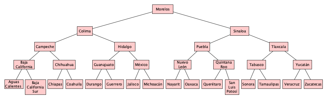
Formally, a (classic) search tree is a tree in which each node is of the form $[t_0 a_1 t_1 a_2 t_2 \ldots a_k t_k]$ where $k \geq 0$ and $a_1$ through $a_k$ comprise an ordered sequence of items (among the items to be searched) and:
- Every node in $t_0$ is less than $a_1$
- Every node in $t_i$ (where $i \in 1 \ldots k-1$) is between $a_i$ and $a_{i+1}$
- Every node in $t_k$ is greater than $a_k$
A picture should help:
Now there are a lot of variations on how we can employ these in practice. For example, we might set minimum and maximum bounds on $k$.
Example: A binary search tree is a classic search tree with $k=1$
Importantly, we may define various kinds of techniques to “rebalance” our tree after insertions and deletions that cause the tree to get too long and skinny. Shorter trees give us the logarithmic search time we crave. Trees that are too long and skinny are sometimes called degenerate trees; here are some examples:
Certain kinds of search trees, like (a,b)-trees, AVL trees, and Red-Black trees, are defined in such a way as to never become degenerate. These trees are covered in separate notes later, but to get a taste of the thinking that goes into making search more efficient in certain cases, here are quick (and of course incomplete) look at at a few of these:
| Tree | Description |
|---|---|
| (a,b) | A search tree having $2 \leq a \leq (b+1)/2$, each internal node except the root having at least $a$ children and at most $b$ children, the root having at most b children, and algorithms for insertion and deletion to keep the tree at minimum height. |
| B | An $(a,b)$ tree with $a = \lceil \frac{b}{2} \rceil$ |
| B+ | A B Tree in which all elements are in leaf nodes, with repeats in internal nodes where necessary. |
| AVL | A binary search tree using the concept of a balance factor to keep the height of the tree ever exceeding $1.45 \log_2 n$. |
| Red Black | A binary search tree in which all nodes are colored red or black, the root is black, all children of a red node are black, and every path from the root to a 0-node or a 1-node has the same number of black nodes. These rules ensure the tree is never taller than $2 \log_2 n$. They provide more efficient insertion and deletion than AVL trees. |
| Scapegoat | A binary search that is simple to implement because it does not need to store heights (like the AVL tree) nor colors (like the Red-Black tree). After a node is inserted that causes an imbalance, we go up the tree to find the scapegoat (where the unbalance is) and completely perfectly rebalance its descendants. |
| Splay | Brings elements up to the top when accessed because irl few elements are accessed most often and recent accesses are likely to be accessed soon. Does not have any height constraints but in practice is (amortized) logarithmic due to access patterns. |
Tries
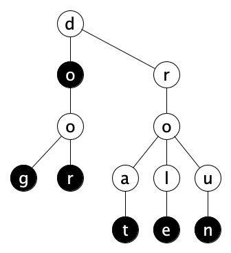
Instead of putting the items to be searched in their own nodes, but we can also spread them out across nodes, in which case our search tree is called a trie, or prefix tree as in this example with the items {do, dog, door, rat, role, run} and an admittedly unrealistic 26-character alphabet, chosen only to make a picture fit on a page:
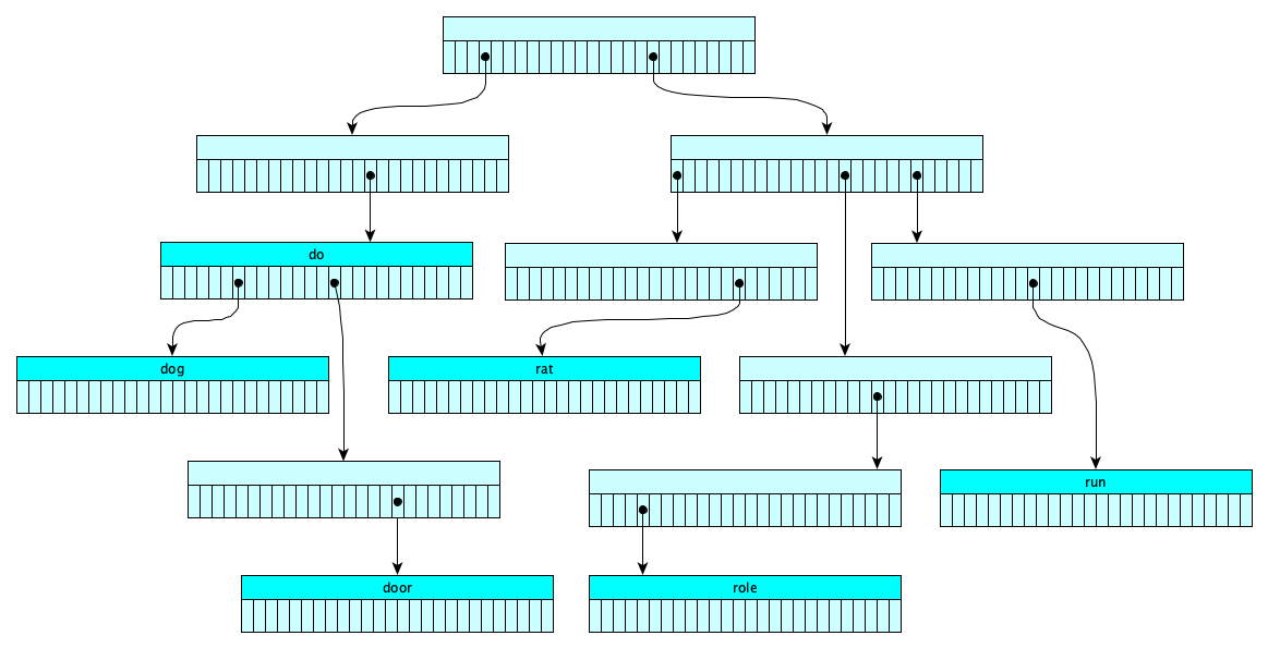
Here search is done character-by-character, but in reality you can encode any data at all into bytes and search byte-by-byte. Each node would then have 256 children, but you can perhaps chunk your data into half-bytes (nybbles) so each node need only 16 children. This would likely save space but make searches twice as long.
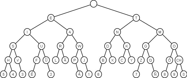
Tries can be space-inefficient: each node has a super wide array of children (many of whose elements are empty). The ternary search tree is a interesting trie implementation that is more compact in terms of space but possibly slower. Here’s an example:
The construction of Ternary Search Trees, along with several examples, will be done interactively in class.
For fun, consider a two-symbol alphabet. Morse code has one! Here the symbols can label the edges (dot for the left, dash for the right), and each node can contain the character at the end of the path:
Spatial Trees
Rather than decomposing the elements themselves into chunks for searching, we sometimes need to find elements in some geographic or temporal region, so we might instead decompose the space that our elements reside in. There are a variety of trees that allow for efficient search for objects located somewhere in space (1-D, 2-D, 3-D, or more dimensions), or even time, or in some other kind of numeric interval. These trees commonly show up as indexes for spatial databases.
The most well-known may be the R-Tree, but you may encounter R*, R+, Quadtrees, Octrees, kd-trees, and many many more. Interval and segment trees solve similar problems. As usual, Wikipedia has a good list.
Summary
We’ve covered:
- How search trees can provide logarithmic search performance
- The two kinds of search trees
- Traditional Search Trees
- Tries
- The fact that trees for spatial indexing exist