The Lambda Calculus

Background

The Lambda Calculus is a theory of functions.

It was created by Alonzo Church around 1930s when he was looking into the foundations of mathematics. It turns out his invention, simple as it is, is actually a universal model of computation.

A good detailed technical overview is David F. Martin’s Notes on the Lambda Calculus. A long textbook chapter overview is Chapter 5 of the Slonneger and Kurtz Book. If you prefer Wikipedia, there’s an article for you there of course. And a really good one at the Stanford Encyclopedia of Philosophy.

If you like videos, here’s a good intro:

Why It Matters

Are you wondering why you’d care about this funny-named theory of functions? (If you said no, you may have had that question answered in the video above, so great!)

The usual answers for “why it matters” and “why study this thing” are that theories are helpful in organizing useful knowledge, and in particular, this Lambda Calculus thing turns out to, even in its simplicity, capture the essence of functions! And as programmers, you know how important functions are to computation. Right? Functions in some sense are what we think of as computation:

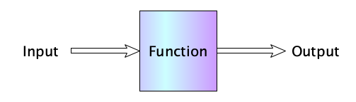
Most modern programming languages have “lambdas” and they are powerful things.

The Basic Idea

If you were making a theory of functions, how simple can you make it? Here’s how Church saw things:

• A function is applied to an (input) argument to compute an (output) result. Examples:

  $\begin{array}{l} \mathtt{square}\;5 \Longrightarrow 25 \\ \mathtt{not}\;\mathtt{true} \Longrightarrow \mathtt{false} \\ \mathtt{factorial}\;8 \Longrightarrow 40320 \end{array}$

• Functions do not have to be named:

  $\begin{array}{l} \lambda x. \mathtt{square}\; (\mathtt{factorial}\;x) \\ \lambda x. \mathtt{not}\; (\mathtt{even}\;x) \\ \lambda x. x \end{array}$

• You compute by reducing terms via function application:

  $\begin{array}{l} (\lambda x. \mathtt{square}\; (\mathtt{factorial}\;x))\;8 \\ \quad\Longrightarrow \mathtt{square}\;(\mathtt{factorial}\;8) \\ \quad\Longrightarrow \mathtt{square}\;40320 \\ \quad\Longrightarrow 1625702400 \end{array}$

• Even though all functions have a single input and a single output, you can simulate a function with multiple inputs by having the function return another function. For example, ($\mathtt{plus}\;3)$ is the function that adds 3 to its argument, so:

  $\begin{array}{l} (\mathtt{plus}\;3)\;5 \Longrightarrow 8 \end{array}$

• If you want to give names to certain terms, you can. Let’s define the name $\mathtt{successor}$ to abbreviate the term $\mathtt{(plus\;1)}$. Then:

  $\begin{array}{l} \mathtt{successor}\;8 \\ \quad\Longrightarrow (\mathtt{plus\;1})\;8 \\ \quad\Longrightarrow 9 \end{array}$

• An aside: function application associates to the left, so $\mathtt{f\;x\;y}$ means $\mathtt{(f\;x)\;y}$. This makes derivations a bit easier to read. Let’s compute whether 317811 is odd:

$\begin{array}{l} (\lambda x. \mathtt{not}\;(\mathtt{eq}\;(\mathtt{mod}\;x\;2)\;0))\;317811 \\ \quad\Longrightarrow \mathtt{not}\;(\mathtt{eq}\;(\mathtt{mod}\;317811\;2)\;0) \\ \quad\Longrightarrow \mathtt{not}\;(\mathtt{eq}\;1\;0) \\ \quad\Longrightarrow \mathtt{not}\;\mathtt{false} \\ \quad\Longrightarrow \mathtt{true} \end{array}$

• And just like functions can be returned from functions, they can also be passed to functions as arguments. The classic example is the famous function twice, defined as:

$ \mathtt{twice} =_{\mathtt{def}} \lambda f. \lambda x. f\;(f\;x) $

By now you should notice that this definition implies:

$\begin{array}{l} \mathtt{twice}\;f = \lambda x. f\;(f\;x) \\ \mathtt{twice}\;f\;x = f\;(f\;x) \end{array}$

Here is an example usage:

$\begin{array}{l} \mathtt{twice}\;\mathtt{square}\;5 \\ \quad\Longrightarrow \mathtt{square}\;(\mathtt{square}\;5) \\ \quad\Longrightarrow \mathtt{square}\;25 \\ \quad\Longrightarrow 625 \end{array}$

and another:

$\begin{array}{l} \mathtt{twice}\;(\lambda x. \mathtt{times}\;5\;x)\;10 \\ \quad\Longrightarrow (\lambda x. \mathtt{times}\;5\;x)\;((\lambda x. \mathtt{times}\;5\;x)\;10) \\ \quad\Longrightarrow (\lambda x. \mathtt{times}\;5\;x)\;( \mathtt{times}\;5\;10) \\ \quad\Longrightarrow (\lambda x. \mathtt{times}\;5\;x)\;50 \\ \quad\Longrightarrow \mathtt{times}\;5\;50 \\ \quad\Longrightarrow 250 \end{array}$

Now it’s time to make a rigorous theory.

The Syntax

The Lambda Calculus is a formal calculus, which means it has a syntax that defines which formulas are legally well-formed (the formal part), and it has rules for transforming one formula into another (the calculus part). Church designed the calculus to mimic what we intuitively think functions should do. Here’s the syntax of the Untyped Applied Lambda Calculus, given with a grammar:

$\begin{array}{lcll} \textit{Exp} & \longrightarrow & \textit{constant} & \\ & | & \textit{variable} & \\ & | & \texttt{"("}\;\textit{Exp}\;\textit{Exp}\;\texttt{")"} & \textrm{--application} \\ & | & \texttt{"("}\;\texttt{"}\mathtt{\lambda}\texttt{"}\;\textit{variable}\;\texttt{"."}\;\textit{Exp}\;\texttt{")"} & \textrm{--abstraction} \\ \end{array}$

You may have guessed from that lead in that there actually exist typed versions of the calculus (“The Typed $\lambda$ Calculus”) as well as non-applied versions (“The Pure $\lambda$ Calculus”). We’ll see those soon. But it’s best to start without types, and with constants. (The pure lambda calculus does not have constants.)

The syntax above is completely unambiguous, thanks to tons of parentheses. In practice, we can remove parentheses as long as we preserve the meaning under the assumptions that (1) the scope of the abstraction’s body goes as far to the right as possible, and (2) application associates to the left.

That might have sounded complicated so we’ll go over these in class:

Official, fully parenthesized expression	Simplified version
$(\mathtt{square}\;5)$	$\mathtt{square}\;5$
$((\mathtt{plus}\;5)\;8)$	$\mathtt{plus}\;5\;8$
$((((x\;y)\;z)\;w)\;x)$	$x\;y\;z\;w\;x$
$(\mathtt{sin}\;(\mathtt{sqrt}\;2))$	$\mathtt{sin}\;(\mathtt{sqrt}\;2)$
$((((x\;y)\;z)\;(w\;y))\;x)$	$x\;y\;z\;(w\;y)\;x$
$(\lambda x. (x\;y))$	$\lambda x. x\;y$
$((\lambda x. x)\;y)$	$(\lambda x. x)\;y$
$(\lambda x. ((x\;y)\;(\lambda z. ((x\;y)\;z))))$	$\lambda x. x\;y\;\lambda z. x\;y\;z$

Here’s the entire abstract syntax:

$\begin{array}{llcl} k: & \mathsf{Constant} & & \\ v: & \mathsf{Variable} & & \\ e: & \mathsf{Expression} & = & k \mid v \mid e\;e \mid \lambda x. e \\ \end{array}$

Vocabulary Time!

Application

An expression of the form $(M\;N)$. Here $M$ is the operator and $N$ is the operand.

Abstraction

An expression of the form $\lambda x. M$. Here $x$ is the parameter and $M$ is the body.

Value

Any expression that is not an application (e.g., a constant, variable, or abstraction).

Values are, well, values.

Applications are like programs, ready to run!

How Does It All Work?

Before we lay out the rules, convince yourself that these three things make sense.

• $\lambda x. \mathtt{hypot}\;x\;3 \Longrightarrow \lambda y. \mathtt{hypot}\;y\;3$
• $(\lambda x.\mathtt{minus}\;x\;1)\;9 \Longrightarrow \mathtt{minus}\;9\;1$
• $\lambda x. \mathtt{square}\;x \Longrightarrow\;\mathtt{square}$

These operations have names:

Example	Name	What it says
$\begin{array}{l}\lambda x. \mathtt{hypot}\;x\;3 \Longrightarrow\\ \quad\lambda y. \mathtt{hypot}\;y\;3\end{array}$	α‑conversion	The name of the variable doesn’t really matter. (Usually)
$\begin{array}{l}(\lambda x.\mathtt{minus}\;x\;1)\;9 \Longrightarrow \\ \quad\mathtt{minus}\;9\;1\end{array}$	β‑conversion	We call functions by passing arguments to parameters, producing the body of the function with the parameter replaced with the argument. (Usually)
$\begin{array}{l}\lambda x. \mathtt{square}\;x \Longrightarrow\\ \quad\mathtt{square}\end{array}$	η‑conversion	You don’t need to wrap a lambda around a perfectly good function. Leave it alone. (Usually)

But why do we say “usually”? This isn’t hard, right? It’s not...hard...is it?

We have to be careful

Any one of these three conversions can go terribly wrong if you don’t do them right. If you naively make changes, the new expression will have a completely different meaning than the original. And that’s bad. Examples:

• $(\lambda x. y) \not\Rightarrow \lambda y. y$   FAILED α
• $(\lambda x. \lambda y. x\;y)\;y \not\Rightarrow \lambda y. y$   FAILED β
• $(\lambda x. x\;x) \not\Rightarrow x$   FAILED η

In the first two cases, the variable $y$ got captured. It became bound when it should have been free. In the third case, $x$ escaped. It was bound and became free. Wait. Bound? Free?

Understanding Bound and Free Variables

The calculus was designed so that:

$\lambda x. \mathtt{plus}\;x\;1$

and:

$\lambda y. \mathtt{plus}\;y\;1$

represent the same thing. In other words, the variable in the abstraction doesn’t really matter too much. We should be able to substitute a different variable, but this does not always work. We cannot substitute $y$ for $x$ in:

$\lambda x. \mathtt{plus}\;x\;y$

Because doing so would change the function from one that “adds its argument to global variable y” to one that “multiplies its argument by two.” Completely different!

How do we make restrictions on this substitution formal? First we define the terms bound and free so that in, say:

$\lambda x. x\;y$

$x$ is bound and $y$ is free. The intuition is that a variable occurrence is bound if it is the variable of an abstraction in the scope of the abstraction and free otherwise.

Remember it’s all about occurrences, not variables

In $((\lambda x. x)\;x)$ we see first the parameter $x$ then two occurrences of $x$. The first occurrence is bound and the second is free. So when asked “which variables are free in this expression” you should understand that question to be asking for occurrences, so don’t just say “$x$”. You need to say which occurrences are free.

That said, some people might call the parameter appearance an “occurrence” and say it’s bound. I guess they are...free...to do so.

Time for examples! Here are a handful of expressions, with the free variables underlined and the bound variables left alone:

• $\underline{x}$
• $\underline{x}\;\underline{y}\;\underline{z}$
• $\lambda x. \underline{y}$
• $\lambda x. x\;\underline{y}$
• $(\lambda x. x)\;\underline{x}$
• $(\lambda x. x\;\underline{y})\;\lambda z. \underline{w}\;\lambda w. w\;z\;\underline{y}\;\underline{x}$

Now we can properly define $\eta$-conversion to avoid escapes:

Rule Name	How it works	Intuition
$\eta$-conversion	$\lambda x. M\;x \Longrightarrow M$   provided that $x \not\in FV(M)$	Bound variables should not become free.

But we need more work to make $\alpha$-conversion and $\beta$-conversion free of captures.

Proper Substitution

$\alpha$ and $\beta$ conversions operate by substituting a variable or an expression for another. But captures are possible if we are not careful. So we have to define proper substitution.

Define the notation $M[N/x]$ to mean the proper substitution of $N$ for all free occurrences of $x$ in $M$, like so:

$E$	$E[M/x]$	Rationale
$k$	$k$	Just a constant, nothing to substitute, leave it alone
$x$	$M$	$x$ is free, and we substitute for free variables, so this is a go
$y$ where $y \neq x$	$y$	This is not the variable we are substituting for, so leave it alone
$(N_1\;N_2)$	$(N_1[M/x]\;N_2[M/x])$	Properly substitute into both terms
$\lambda x. N$	$\lambda x. N$	$x$ is bound, you cannot substitute for it! Leave it alone.
$\lambda y. N$ where $y \neq x$	if $x\not\in FV(N)$ $\quad \lambda y. N$ else if $y\not\in FV(M)$ $\quad \lambda y. N[M/x]$ else $\quad \lambda z.((N[z/y])[M/x])$ $\quad\quad$ where $z$ is a new $\quad\quad$variable not free $\quad\quad$in $M$ nor $N$	Case 1: no free $x$, ignore. Case 2: there is no free $y$ in $M$ that will be captured, substitution is safe. Case 3: we have to avoid $y$ getting captured, so first, rename $y$ to a new fresh $z$ before substituting for $x$. By fresh we mean one that will not itself capture anything in $M$ or $N$.

Practice!

• $\mathsf{times}[2/x] \equiv \mathsf{times}$
• $x[2/x] \equiv 2$
• $y[2/x] \equiv y$
• $(f\;x)[2/x] \equiv f\;2$
• $(x\;y)[2/x] \equiv 2\;y$
• $(x\;x)[z/x] \equiv z\;z$
• $((g\;x)\;x)[2/x] \equiv g\;2\;2$
• $(\lambda x. f\;x\;y)[2/x] \equiv \lambda x. f\;x\;y$
• $(\lambda x. f\;x\;y)[z/x] \equiv \lambda x. f\;x\;y$
• $(\lambda y. f\;x\;y)[z/x] \equiv \lambda y. f\;z\;y$
• $(\lambda y. f\;x\;y)[y/x] \equiv (\lambda z. f\;x\;z)[y/x] \equiv\lambda z. f\;y\;z$

This is good enough for $\beta$-conversion, but $\alpha$-conversion needs a qualifier:

Rule Name	How it works	Intuition
$\alpha$-conversion	$\lambda x. M \Longrightarrow \lambda y. M[y/x]$    provided that $y \not\in FV(M)$	We cannot rename $x$ to $y$ if $y$ is free in $M$ because the free $y$ would get captured
$\beta$-conversion	$(\lambda x. M)\;N \Longrightarrow M[N/x]$	There are no fancy provisos on this rule, because substitution itself has been defined to avoid capture.

Reduction

Computation proceeds by reducing expressions, specifically applications. There are two kinds of reductions:

• Beta-reduction: $(\lambda x. M)\;N \Longrightarrow M[N/x]$
• Constant application: For expressions like $(\texttt{sqrt}\;100)$, carry out whatever computation the constant operator is defined to mean.

An expression that can be reduced is a reducible expression: a redex.

When you’ve reduced an expression to the point where no reduction operations can be applied any more, you’ve reached the normal form of the expression.

Not every expression has a normal form. Here’s one that doesn’t: $(\lambda x. x\;x)\;(\lambda x. x\;x)$. Some people call this $\Omega$.

When you perform reductions, you sometimes have a choice of which part of an expression you want to reduce first. Example:

• $(\lambda x. x + x)(3 \times 5) \Longrightarrow (3 \times 5) + (3 \times 5)$
• $(\lambda x. x + x)(3 \times 5) \Longrightarrow (\lambda x. x + x)(15)$

Can different choices of what to reduce next lead to different normal forms? Nope. It turns out that every expression has at most one normal form, and that normal form is unique, up to the names of its bound variables, anyway. This is a corollary to the famous Church-Rosser Theorem. The theorem is actually: For every lambda expression $E$, $M_1$, and $M_2$, if $E \Longrightarrow^* M_1$ and $E \Longrightarrow^* M_2$, then there exists an expression $N$ such that $M_1 \Longrightarrow^* N$ and $M_2 \Longrightarrow^* N$.

This choice gives rise to two different semantics:

The Call-By-Value (CBV) Lambda Calculus

You cannot do any reductions unless the operand is a value, and you cannot perform any reductions inside the body of an abstraction.

The Call-By-Name (CBN) Lambda Calculus

You have to apply the functions as soon as possible (don’t evaluate the operand!)

Note how both of these restrict the anything-goes basic semantics.

How is this related to programming languages?

Most programming languages use call-by-value. But some languages, like Haskell, use call-by-name. And some languages might even let you choose.

Here’s a CBV Reduction:

$\begin{array}{l} (\lambda x. x + x)((\lambda x. 3x + 1) 5) \\ \quad\Longrightarrow (\lambda x. x + x)(3 \times 5 + 1) \\ \quad\Longrightarrow (\lambda x. x + x)(16) \\ \quad\Longrightarrow 16 + 16 \\ \quad\Longrightarrow 32 \end{array}$

And here’s a CBN Reduction:

$\begin{array}{l} (\lambda x. x + x)((\lambda x. 3x + 1) 5) \\ \quad\Longrightarrow (\lambda x. 3x + 1)5 + (\lambda x. 3x + 1)5 \\ \quad\Longrightarrow (3 \times 5 + 1) + (\lambda x. 3x + 1)5 \\ \quad\Longrightarrow 16 + (\lambda x. 3x + 1)5 \\ \quad\Longrightarrow 16 + (3 \times 5 + 1) \\ \quad\Longrightarrow 16 + 16 \\ \quad\Longrightarrow 32 \end{array}$

Same normal form!

The two different calculi are sometimes confused with two reduction strategies. These are:

The Normal Order Reduction Strategy (NORS)

Always reduce the leftmost, outermost redex first.

The Applicative Order Reduction Strategy (AORS)

Always reduce the leftmost, innermost redex first.

Lambdas IRL

Most major programming languages have “lambdas” a.k.a “anonymous functions.” Let’s start easy, with the square function:

Language	The Square Function
JavaScript	x => x ** 2
TypeScript	(x: number): number => x ** 2
Python	lambda x: x ** 2
Ruby	->(x) {x ** 2}
Lua	function (x) return x ^ 2 end
Kotlin	{x: Double -> x * x}
Swift	{$0 as Double * $0}
Rust	|x| {x * x}
Perl	{ $_ * $_ }
Java	(x) -> x * x
C++	[](double x) {return x * x;}
C#	x => x * x
F#	fun x -> x * x
Go	func(x float64)float64 {return x * x}
Julia	x -> x^2
Gleam	fn(x) { x * x }
Lisp	(lambda (x) (* x x))
Clojure	#(* % %)
Haskell	\x -> x ^ 2
Scala	(x: Double) => x * x
PHP	fn($x) => $x ** 2
Dart	(double x) => x * x
R	\(x) x ^ 2
Elixir	fn x -> x * x end
K	{x^2}
Factor	[ dup * ]

Lambdas show up a lot when used with functions like map, filter, and reduce. Here are examples of how different languages specify a function to compute the sum of the squares of the even numbers of a list (H/T Xan Mavromatis for writing a few of these):

function sumOfEvenSquares(a) {
  return a
    .filter(x => x % 2 === 0)
    .map(x => x ** 2)
    .reduce((x, y) => x + y, 0)
}

def sum_of_even_squares(a):
    return sum(x*x for x in a if x % 2 == 0)

def sum_of_even_squares(a)
  a.select{|x| x % 2 == 0}.map{|x| x * x}.reduce(0, :+)
end

fun sumOfEvenSquares(a: Array<Int>): Int {
    return a.filter { it % 2 == 0 }.map { it * it }.sum()
}

func sumOfEvenSquares(of a: [Int]) -> Int {
    return a.filter{$0 % 2 == 0}.map{$0 * $0}.reduce(0, +)
}

fn sum_of_even_squares(a: &[i32]) -> i32 {
    a.iter()
        .filter(|&&x| x % 2 == 0)
        .map(|&x| x * x)
        .sum()
}

sub sum_of_even_squares {
    sum0 map { $_**2 } grep { $_ % 2 == 0 } @_;
}

public static int SumOfEvenSquares(int[] a) {
    return IntStream.of(a).filter(x -> x % 2 == 0).map(x -> x * x).sum();
}

// Must use System.Linq
public static int SumOfEvenSquares(int[] a)
{
    return a.Where(x => x % 2 == 0).Select(x => x * x).Sum();
}

(defn sum-of-even-squares [a]
  (->> a (filter even?) (map #(* % %)) (reduce +)))

proc sum_of_even_squares(a) {
  return + reduce ([x in a] if x % 2 == 0 then x*x else 0);
}

function sumOfEvenSquares(a)
    sum(x -> x^2, filter(x -> x % 2 == 0, a), init = 0)
end

sumOfEvenSquares :: [Int] -> Int
sumOfEvenSquares = sum . map (^ 2) . filter even

let sum_of_even_squares a =
    a
    |> List.filter (fun x -> x % 2 = 0)
    |> List.sumBy (fun x -> x * x)

sumofevensquares: {+/x[&~x!2]^2}

Some languages, notably Lua and Verse, don’t seem to have native approaches to mapping, filtering, and reducing for their higher-order functions.

The Pure λ-Calculus

Believe it or not, we can build up all the constants of mathematics from lambda expressions. You don’t need numbers or booleans or lists or anything, all you need are functions. Nothing but functions. You get the objects you need by defining them to be...functions! Here are a few:

$\begin{array}{l} 0 =_{\mathtt{def}} \lambda f. \lambda x. x \\ 1 =_{\mathtt{def}} \lambda f. \lambda x. f\;x \\ 2 =_{\mathtt{def}} \lambda f. \lambda x. f\;(f\;x) \\ 3 =_{\mathtt{def}} \lambda f. \lambda x. f\;(f\;(f\;x)) \\ 4 =_{\mathtt{def}} \lambda f. \lambda x. f\;(f\;(f\;(f\;x))) \\ \vdots \end{array}$

The number $n$ is a function that takes in a function $f$ and some $x$ and applies $f$ $n$ times to $x$ (or, in the notation you are used to: $f^n(x)$). So this means:

$ \mathtt{successor} =_{\mathtt{def}} \lambda n. \lambda f. \lambda x. f\;(n\;f\;x) $

And then $\mathtt{plus}\;m\;n$ is applying the successor function $m$ times to $n$:

$ \mathtt{plus} =_{\mathtt{def}} \lambda m. \lambda n. m\;\mathtt{successor}\;n $

with multiplication following from that in a straightforward way:

$ \mathtt{times} =_{\mathtt{def}} \lambda m. \lambda n. m\;(\mathtt{plus}\;n)\;0 $

Interestingly, addition and multiplication can be simplified:

$\begin{array}{l} \mathtt{plus} =_{\mathtt{def}} \lambda m. \lambda n. \lambda f. \lambda x. m\;f\;(n\;f\;x)\\ \mathtt{times} =_{\mathtt{def}} \lambda m. \lambda n. \lambda f. m\;(n\;f) \end{array}$

And amazingly, exponentiation turns out to be just this:

$\mathtt{pow} =_{\mathtt{def}} \lambda b. \lambda e. e\;b$

How about Booleans?

$\begin{array}{l} \mathtt{true} =_{\mathtt{def}} \lambda x. \lambda y. x \\ \mathtt{false} =_{\mathtt{def}} \lambda x. \lambda y. y \\ \mathtt{not} =_{\mathtt{def}} \lambda p. p\;\mathtt{false}\;\mathtt{true} \\ \mathtt{and} =_{\mathtt{def}} \lambda p. \lambda q. p\;q\;p \\ \mathtt{or} =_{\mathtt{def}} \lambda p. \lambda q. p\;p\;q \\ \mathtt{ifthenelse} =_{\mathtt{def}} \lambda r. \lambda p. \lambda q. r\;p\;q \end{array}$

Ordered pairs:

$\begin{array}{l} \mathtt{pair} =_{\mathtt{def}} \lambda x. \lambda y. \lambda f. f\;x\;y \\ \mathtt{first} =_{\mathtt{def}} \lambda p. p\;\mathtt{true} \\ \mathtt{second} =_{\mathtt{def}} \lambda p. p\;\mathtt{false} \\ \end{array}$

A list is either empty or the prefixing of an item (its head) and a list (its tail). The simplest list is the empty list, structurally the same as both $0$ and $\mathtt{false}$:

$ \mathtt{emptylist} =_{\mathtt{def}} \lambda c. \lambda n. n $

Non empty lists are formed with the prefixing function that people call $\texttt{cons}$:

$\mathtt{cons} =_{\mathtt{def}} \lambda x. \lambda y. \lambda c. \lambda n. c\;x\;(y\;c\;n)$

Lists have a sugared form:

$\begin{array}{ll} (\mathtt{cons} \;x\; \mathtt{emptylist}) & \textrm{is sugared as } [x] \\ (\mathtt{cons} \;x\; (\mathtt{cons} \;y\; \mathtt{emptylist})) & \textrm{is sugared as } [x,y] \\ (\mathtt{cons} \;x\; (\mathtt{cons} \;y\; (\mathtt{cons} \;z\; \mathtt{emptylist}))) & \textrm{is sugared as } [x,y,z] \end{array}$

Sets are functions that when given an argument, return $\mathtt{true}$ if the argument is in the set and $\mathtt{false}$ otherwise.

$\begin{array}{l} \mathtt{emptyset} =_{\mathtt{def}} \lambda x. \mathtt{false} \\ \mathtt{universalset} =_{\mathtt{def}} \lambda x. \mathtt{true} \\ \mathtt{is\_member} =_{\mathtt{def}} \lambda s. \lambda x. s\;x \\ \mathtt{union} =_{\mathtt{def}} \lambda s. \lambda t. \lambda x. \mathtt{or}\;(s\;x)\;(t\;x) \\ \mathtt{intersection} =_{\mathtt{def}} \lambda s. \lambda t. \lambda x. \mathtt{and}\;(s\;x)\;(t\;x) \\ \end{array}$

You can keep going, defining an unlimited number of arithmetic, logical, and other functions using just the lambda calculus. To make things readable, you are free to use crazy mathematical notation like infix operators with funny symbols. Here are some examples:

Standard Form	Sugared Form
($\texttt{successor}$ $x$)	$x + 1$
($\texttt{plus}$ $x$ $y$)	$x + y$
($\texttt{minus}$ $x$ $y$)	$x - y$
($\texttt{times}$ $x$ $y$)	$x \times y$
($\texttt{divide}$ $x$ $y$)	$x \div y$
($\texttt{remainder}$ $x$ $y$)	$x \;\mathtt{\%}\; y$
($\texttt{pow}$ $x$ $y$)	$x^y$
($\texttt{tetrate}$ $x$ $y$)	$x \uparrow\uparrow y$
($\texttt{pentate}$ $x$ $y$)	$x \uparrow\uparrow\uparrow y$
($\texttt{negate}$ $x$)	$-x$
($\texttt{sqrt}$ $x$)	$\sqrt{x}$
($\texttt{factorial}$ $x$)	$x!$
($\texttt{exp}$ $x$)	$e^x$
($\texttt{floor}$ $x$)	$\lfloor x \rfloor$
($\texttt{ceil}$ $x$)	$\lceil x \rceil$
($\texttt{less}$ $x$ $y$)	$x \lt y$
($\texttt{lesseq}$ $x$ $y$)	$x \leq y$
($\texttt{eq}$ $x$ $y$)	$x = y$
($\texttt{noteq}$ $x$ $y$)	$x \not= y$
($\texttt{greater}$ $x$ $y$)	$x > y$
($\texttt{greatereq}$ $x$ $y$)	$x \geq y$
($\texttt{not}$ $x$)	$\neg x$
($\texttt{and}$ $x$ $y$)	$x \wedge y$
($\texttt{or}$ $x$ $y$)	$x \vee y$
($\texttt{pair}$ $x$ $y$)	$(x, y)$
($\texttt{pair}$ $x$ ($\texttt{pair}$ $y$ $z$))	$(x, y, z)$
$\texttt{emptylist}$	$[\,]$
($\texttt{cons}$ $x$ emptylist)	$[x]$
($\texttt{cons}$ $x$ ($\texttt{cons}$ $y$ emptylist))	$[x,y]$
($\texttt{cons}$ $x$ ($\texttt{cons}$ $y$ ($\texttt{cons}$ $z$ emptylist)))	$[x,y,z]$
$\texttt{emptyset}$	$\varnothing $
($\mathtt{is\_member}$ $s$ $x$)	$x \in s$
($\texttt{union}$ $s$ $t$)	$s \cup t$
($\texttt{intersection}$ $s$ $t$)	$s \cap t$

You can even start to make these lambda-expressions look like a programming language! When you apply a function to an argument, you are LET-ting the parameter be the argument within the body of the function. So writing the application:

$(\lambda x. x + 5)\;3$

could be written as:

$\mathsf{let}\;x=3\;\mathsf{in}\;(x + 5)$

We sometimes see it written as this as well:

$(x + 5)\;\mathsf{where}\;x=3$

All three of these are the same $\lambda$-expression. The symbols $\mathsf{let}$, $\mathsf{in}$, and $\mathsf{where}$ are symbols of the sugared $\lambda$ Calculus itself; they are not constants!

Another convenient form is:

$\mathsf{if}\;E_1\;\mathsf{then}\;E_2\;\mathsf{else}\;E_3$

which sugars $(\texttt{ifthenelse}\;E_1\;E_2\;E_3)$. You can use it in a computation as in this example:

$\begin{array}{l} \;\; (\lambda x. \mathsf{if}\;x \lt 3\;\mathsf{then}\;2 \times x\;\mathsf{else}\;x+5)\;10 \\ \quad\;\; \Longrightarrow \mathsf{if}\;10 \lt 3\;\mathsf{then}\;2 \times 10\;\mathsf{else}\;10+5 \\ \quad\;\; \Longrightarrow \mathsf{if}\;\mathsf{false}\;\mathsf{then}\;2 \times 10\;\mathsf{else}\;10+5 \\ \quad\;\; \Longrightarrow 10+5 \\ \quad\;\; \Longrightarrow 15 \end{array}$

Recursion

The Lambda Calculus can do booleans, logic, numbers, arithmetic, function invocation, and even conditional evaluation. But can it do iteration (i.e., loops and recursion)?

Why It Is Hard

How can we define the factorial function? First note this does NOT work:

$\;\; \mathtt{fact} \equiv_{\mathtt{def}} \lambda n. \mathsf{if}\;n=0\;\mathsf{then}\;1\;\mathsf{else}\;n \times \mathtt{fact}(n-1)$

We’re trying to define fact but assuming it already exists? That’s not right! We have to evaluate the right hand side first, then bind it to fact.

Perhaps what was meant was:

$\begin{array}{l} \mathtt{fact} \equiv_{\mathtt{def}} \\ \quad\;\; \lambda n. \mathsf{if}\;n=0\;\mathsf{then}\;1\;\mathsf{else}\;x \times (\lambda n. \mathsf{if}\;n=0\;\mathsf{then}\;1\;\mathsf{else}\;x \times \ldots)(n-1) \end{array}$

which is nonsense. We can’t have infinitely long expressions. The whole point of computation is to find finite representations (programs, functions, what have you) of things.

What we want is something like this:

$\begin{array}{l} \mathtt{fact} \equiv_{\mathtt{def}} \\ \quad\;\; \textrm{the function}\;f\;\textrm{such that}\;f = \lambda n. \mathsf{if}\;n=0\;\mathsf{then}\;1\;\mathsf{else}\;x \times f(n-1) \end{array}$

But how do we possibly find such an $f$? What sorcery is required?

Fixpoints

This is wild indeed so hang on. How do we deal with these “such that” questions? How do we find values that “satisfy” statements? Sometimes we can just guess:

• The $x$ such that $x = \cos x$ is $0.73908513321516064166\ldots$
• The $x$ such that $x = x^0$ is $1$
• The $x$ such that $x = 6-x^2$ is $2$. Or $-3$.

How do we make this more rigorous? We use the idea of a fixpoint. A fixpoint of a function $f$ is a value $x$ such that $f(x)=x$. That’s it. That’s all it is. Examples are helpful:

Function	Fixpoints
$\lambda x. \cos x$	$0.73908513321516064166\ldots$
$\lambda x. x^0$	$1$
$\lambda x. 6-x^2$	$2$ $-3$
$\lambda x. x!$	$0$ $1$
$\lambda x. x^2-x$	$0$ $2$
$\lambda x. x$	all values are fixpoints
$\lambda x. x + 1$	no fixpoints (well JS has NaN)

Now, if there existed a function, called, say, fix, that would find fixpoints of a function for us, then we could write:

$\begin{array}{l} \mathtt{fact} \equiv_{\mathtt{def}} \\ \quad\;\; \mathtt{fix}\;\lambda f. \lambda n. \mathsf{if}\;n=0\;\mathsf{then}\;1\;\mathsf{else}\;n \times f(n-1) \end{array}$

See why? Because what is the fixpoint of $\lambda f. \lambda n. \mathsf{if}\;n=0\;\mathsf{then}\;1\;\mathsf{else}\;n \times f(n-1)$? It’s the function $f$ such that.... You get the idea.

The Trick

Now how do we write fix? First, understand what it is supposed to do. $\mathtt{fix}\;f$ must produce a fixpoint of $f$, namely some value for which $x = f(x)$. So that means that fix must satisfy the equation:

$ \mathtt{fix}\;f = f(\mathtt{fix}\;f) $

How even can we find what fix is? Well someone did, and they called it $Y$:

$ Y \equiv_{\mathrm{def}} \lambda f. (\lambda g. (f\;(g\;g))\;\lambda g.(f\;(g\;g))) $

Wait, what? Seriously? Let’s see:

$\begin{array}{l} Y\;f & = & \lambda g. (f\;(g\;g))\;\lambda g.(f\;(g\;g)) \\ & = & f\;(\lambda g.(f\;(g\;g))\;\lambda g.(f\;(g\;g))) \\ & = & f\;(Y\;f) \end{array}$

🤯

This so-called Y-combinator gives you fixed points only in the call-by-name calculus. You need a different one, $Z$, for the call-by-value calculus.

$ Z =_{\mathrm{def}} \lambda f.(\lambda g.(f\;\lambda h.((g\;g)\;h))\;\lambda g.(f\;\lambda h.((g\;g)\;h))) $

Why This Matters

This is awesome because now we have justified the use of recursion as a proper computational mechanism! Yes, that is a big deal.

Let’s see it in action with factorial. We are going to define:

$\begin{array}{l} \mathtt{fact} =_{\mathtt{def}} \\ \quad\;\; Y\;\lambda f. \lambda n. \mathsf{if}\;n=0\;\mathsf{then}\;1\;\mathsf{else}\;x \times f(n-1) \end{array}$

This is a proper definition because we are not using fact to define fact. We are in the clear. But does it actually work? Let’s try it. Let’s compute $\mathtt{fact}\;3$. Because these derivations can get really long, we’ll use $F$ to stand for the expression $\lambda f. \lambda n. \mathsf{if}\;n=0\;\mathsf{then}\;1\;\mathsf{else}\;n \times f(n-1)$. Here goes:

$\begin{array}{l} \mathtt{fact}\;3 & = & Y\;F\;3 \\ & = & F\;(Y\;F)\;3 \\ & = & ((\lambda f. \lambda n. \mathsf{if}\;n=0\;\mathsf{then}\;1\;\mathsf{else}\;n \times f(n-1))(Y\;F))\;3 \\ & = & \mathsf{if}\;3=0\;\mathsf{then}\;1\;\mathsf{else}\;3 \times (Y\;F)(3-1) \\ & = & 3 \times (Y\;F)(2) \\ & = & 3 \times ((\lambda f. \lambda n. \mathsf{if}\;n=0\;\mathsf{then}\;1\;\mathsf{else}\;n \times f(n-1))(Y\;F))(2) \\ & = & 3 \times (\mathsf{if}\;2=0\;\mathsf{then}\;1\;\mathsf{else}\;2 \times (Y\;F))(2-1) \\ & = & 3 \times 2 \times (Y\;F)(1) \\ & = & 3 \times 2 \times 1 \times (Y\;F)(0) \\ & = & 3 \times 2 \times 1 \times 1 \\ & = & 6 \\ \end{array}$

Combinators

Did you wonder why we said “Y combinator” and “Z combinator” above?

There is a word for an lambda expression with no free variables: combinator. Combinators are convenient since using them means you have less variables floating around, so your expressions are simpler. And you can get good at working only on the level of the combinators, combining them to form powerful operators.

Here’s a list of some well-known combinators:

Comb	Name	Definition	Alt Def	Facts
$M$	Mockingbird	$\lambda x. x\;x$	$SII$	$Mx = xx$
$I$	Identity Bird	$\lambda x. x$	$SKK$	$Ix = x$
$K$	Kestrel	$\lambda x. \lambda y. x$		$Kxy = x$
$T$	Thrush	$\lambda x. \lambda y. y\;x$	$CI$	$Txy = yx$
$W$	Warbler	$\lambda x. \lambda y. x\;y\;y$	$C(BMR)$	$Wxy = xyy$
$L$	Lark	$\lambda x. \lambda y. x\;(y\;y)$	$CBM$	$Lxy = x(yy)$
$O$	Owl	$\lambda x. \lambda y. y\;(x\;y)$	$SI$	$Oxy = y(xy)$
$U$	Turing	$\lambda x. \lambda y. y\;(x\;x\;y)$	$LO$	$Uxy = y(xxy)$
$S$	Starling	$\lambda x. \lambda y. \lambda z. x\;z\;(y\;z)$		$Sxyz = xz(yz)$
$B$	Bluebird	$\lambda x. \lambda y. \lambda z. x\;(y\;z)$	$S(KS)K$	$Bxyz = x(yz)$
$R$	Robin	$\lambda x. \lambda y. \lambda z. y\;z\;x$	$BBT$	$Rxyz = yzx$
$C$	Cardinal	$\lambda x. \lambda y. \lambda z. x\;z\;y$	$RRR$	$Cxyz = xzy$
$V$	Vireo	$\lambda x. \lambda y. \lambda z. z\;x\;y$	$BCT$	$Vxyz = zxy$
$D$	Dove	$\lambda x. \lambda y. \lambda z. \lambda w. x\;y\;(z\;w)$	$BB$	$Dxyzw = xy(zw)$
$B_1$	Blackbird	$\lambda x. \lambda y. \lambda z. \lambda w. x\;(y\;z\;w)$	$BBB$	$B_1xyzw = x(yzw)$
$E$	Eagle	$\lambda x. \lambda y. \lambda z. \lambda w. \lambda v. x\;y\;(z\;w\;v)$	$B(BBB)$	$Exyzwv = xy(zwv)$
$KI$	Kite	$\lambda x. \lambda y. y$	$KI$	$KIxy = Iy = y$

Combinators form the basis of point-free programming and are the basis of concatenative programming languages.

If you are interested in this point-free, stuff, here’s the first of an entire video series called...Point-Free.

BIRDS!

You really need to read Raymond Smullyan’s To Mock a Mockingbird. Smullyan, like Turing, was a PhD student of Church’s. So was Kleene, Martin, Rosser, Rabin, Scott, Andrews, Davis. Woah.

Amazing Fun Fact

You can create every possible combinator from just $S$ and $K$.

More vocabulary: You can also call a combinator (an expression without free variables) a closed expression, and an expression with free variables an open expression.

The Typed λ-Calculus

Church invented all this in the first place not to build a programming language, but to find a foundation for mathematics itself, in the spirit of Frege, Russell, and Whitehead. It seemed to work great: the “nothing but functions” approach encodes numbers, booleans, pairs, lists, logical ands and ors and nots, sets, and more, just with abstraction and application.

But it didn’t exactly work, because Russell’s Paradox showed up. Because sets are just functions that return $\mathtt{true}$ or $\mathtt{false}$ depending on whether an argument is in the set, the set of all sets that are not members of themselves, which we’ll call $R$, is defined like this:

$ R =_{\mathtt{def}} \lambda x. \neg(x\;x) $

Let’s see if $R \in R$:

$\begin{array}{l} R\;R \\ \quad = (\lambda x. \neg(x\;x))\;R \\ \quad \Longrightarrow \neg(R\;R) \end{array}$

That’s fine as computation goes, but terrible for logic, and terrible as a foundation for mathematics!

Whitehead and Russell’s got around this problem in Principia Mathematica by introducing a hierarchy of types so that “$x \in x$” could not even be formed as a well-typed statement in the first place. Church still wanted his foundation for mathematics, so he also turned to types.

Church’s Simply-Typed Lambda Calculus

Church introduced types into the Lambda Calculus in his famous 1940 paper “A Formulation of the Simple Theory of Types.” The system is composed of:

Church then introduced logical constants and operators, and even numerals, as abbreviations. Here’s a screenshot from the paper, showing the old-fashioned notation of logical formulas in bold, logical and represented with juxtaposition, and implicit $\forall$ quantifier:

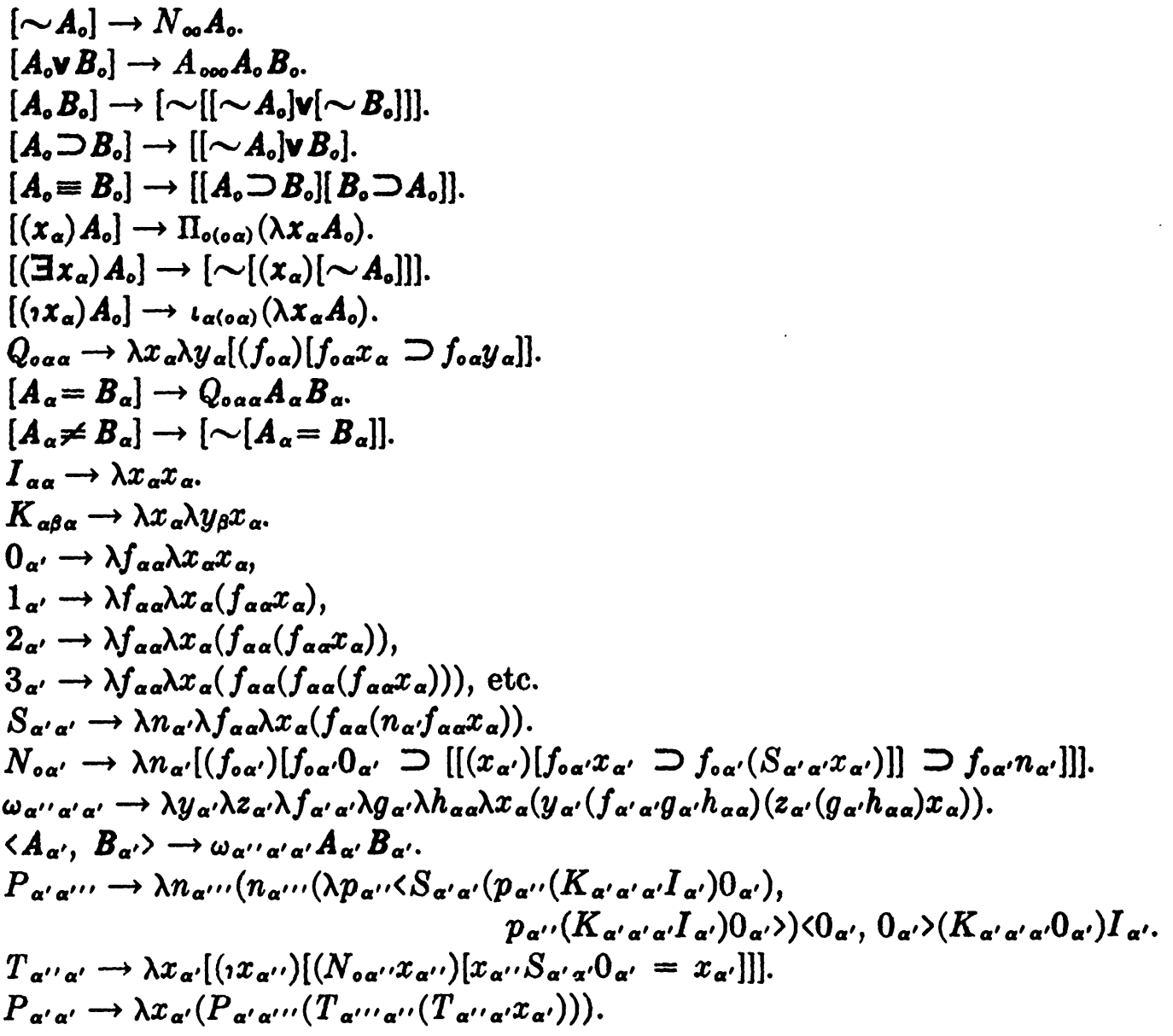
To make the system work as a logic, he introduced 11 axioms and 6 inference rules, which appear on pages 60 and 61 of the paper. Do make sure to read the full paper to complete your understanding of the system.

The Simple Type Theory is not Turing Complete

Types remove the problem of Russell’s Paradox by blocking the self-referential $\lambda x. \neg(x\;x)$, but as this also blocks the fixpoint combinators from the Recursion section ($Y$ and $Z$ are themselves built from self-application) so the STLC isn’t Turing-complete. In practice, modern programming languages use a combination of types and recursion to get the best of both worlds.

The Lambda Cube

There are several different formulations of type theories based on the Lambda Calculus. Church’s was the first. It is called a simple type theory. What’s a simple type theory?

If you only have a type of individuals and a type of truth values, you have a simple type theory. If you add products, sums, and even natural numbers, it’s still simple. If you add recursion, yeah, most people might still call it simple. Once you add polymorphic types or dependent types, you are no longer simple.

Henk Barendregt, who one could call a true expert-guru-wizard authority on lambda calculus, did an amazing classification of typed lambda calculi known as the Lambda Cube. The idea is that the base calculus can be extended in three ways, allowing...

• types to depend on terms (dependent types)
• terms to depend on types (polymorphic types)
• types to depend on types (type operators)

...and if you show these extensions as axes of a cube, you can describe 8 different calculi.

We’ll look at the three axes, and the 8 systems via the Wikipedia article, which has a good presentation.

You can read about the Lambda Cube at Wikipedia. It’s beneficial to first read the articles on Typed lambda calculi and the OG simply-typed lambda calculus.

Recall Practice

Here are some questions useful for your spaced repetition learning. Many of the answers are not found on this page. Some will have popped up in lecture. Others will require you to do your own research.

1. Who invented the Lambda Calculus and why?
   Alonzo Church, to study the foundations of mathematics and computation.
2. What is the Lambda Calculus most concerned with?
   Functions.
3. In the Lambda Calculus, can functions have more than one parameter? More than one result?
   No and no. One parameter only. One result only.
4. Why are computer scientists interested in the Lambda Calculus as a foundational theory?
   Functions are dynamic and feel more like computation. Sets are kind of just static.
5. What is the main thing you do with functions?
   Apply them to arguments.
6. How do we write the application of function $f$ to argument $x$?
   Officially $(f\;x)$, but it is perfectly fine to write $f\;x$ or even $f(x)$.
7. Write two distinct lambda expressions for averaging two numbers, one using tuples and one that does not. Assume that there are pre-defined constants $\texttt{plus}$ and $\texttt{divide}$, as well as constants for all numbers.
   $\lambda x. \lambda y. \texttt{divide}\;(\texttt{plus}\;x\;y)\;2$
   $\lambda (x,y). \texttt{divide}(\texttt{plus}(x,y),2)$
8. What are the four types of expressions in the untyped applied Lambda Calculus?
   Variables, Constants, Applications, Abstractions.
9. The expression $\lambda x. f\;(\lambda x. g\;y\;\lambda y. g)\;x\;y$ is a syntactic abbreviation for which proper expression?
   $(\lambda x. ((f\;(\lambda x. ((g\;y)\;(\lambda y. g)))\;x)\;y))$
10. The expression $x\;\lambda y. y\;x$ is a syntactic abbreviation for which proper expression?
    $(x\;(\lambda y. (y\;x)))$
11. What is a value in the Lambda Calculus?
    An expression that is not an application.
12. What are the two parts of an application called?
    The operator and the operand.
13. What is the syntax of an abstraction?
    $(\lambda x. E)$
14. What are the two parts of an abstraction called?
    The parameter and the body.
15. What are three conversions in Lambda Calculus computation?
    Alpha, Beta, Eta.
16. Which conversion deals with renaming parameters?
    Alpha
17. Which conversion deals with applying functions to arguments?
    Beta
18. Which conversion deals with removing needless abstractions?
    Eta
19. What can happen if $\alpha$-conversion or $\beta$-conversion is applied without taking into account its restrictions?
    Free variables can become bound.
20. What can happen if $\eta$-conversion is applied without taking into account its restrictions?
    Bound variables can become free.
21. What is a capture? What is an escape?
    A capture is when a free variable becomes bound. An escape is when a bound variable becomes free.
22. What someone says “Which are the free variables in this expression?” what do they really mean?
    They are asking “Which variable OCCURRENCES are free in this expression?”
23. Is $\texttt{plus}$ free in $\lambda y. \mathtt{plus}\;y\;1$? Why or why not?
    No, because it is a constant.
24. Which occurrences of $x$ are free in $(\lambda x. \lambda y. x\;y)\;x$?
    The last one only.
25. How do you read $E_1[E_2/x]$?
    The proper substitution of $E_2$ for all free occurrences of $x$ in $E_1$.
26. Perform the substitution $(\lambda y. f\;x\;y)[y/x]$.
    $(\lambda z. f\;y\;z)$
27. What is a redex?
    A reducible expression.
28. What is a normal form?
    An expression that cannot be reduced further.
29. What is interesting about the expression $(\lambda x. x\;x)\;(\lambda x. x\;x)$?
    It has no normal form.
30. Can an expression have more than one normal form?
    No, not really. They are all essentially the same, differing only in the names of bound variables.
31. What characterizes the call-by-value calculus?
    Arguments are evaluated before the function is applied, and you may not reduce inside the body of an abstraction.
32. What characterizes the call-by-name calculus?
    Arguments are not evaluated before the function is applied.
33. What are two well-known reduction strategies?
    Normal order (NORS) and applicative order (AORS).
34. How do NORS and AORS differ?
    NORS reduces the leftmost, outermost redex first. AORS reduces the leftmost, innermost redex first.
35. How do the applied and pure Lambda Calculi differ?
    The applied Lambda Calculus has constants, while the pure Lambda Calculus does not.
36. How are true and false represented in the Pure Lambda Calculus?
    $\lambda x. \lambda y. x$ and $\lambda x. \lambda y. y$
37. How do we represent the natural number $n$ in the Pure Lambda Calculus?
    $\lambda f. \lambda x. f^n\;x$
38. How do you write $\textsf{let}\;x=1\;\textsf{in}E$ in the Lambda Calculus?
    $(\lambda x. E)\;1$
39. How do you write the list $[1,2,3]$ in the Lambda Calculus (it’s ok to use function iteration notation)?
    $(\texttt{pair}\;1\;(\texttt{pair}\;2\;(\texttt{pair}\;3\;\texttt{emptylist})))$
40. Why is recursion “hard” in the Lambda Calculus?
    You can’t define a function in terms of itself.
41. How do we get the effect of recursion in the Lambda Calculus?
    Fixpoint combinators.
42. What is a fixpoint of a function $f$?
    A value $x$ such that $f(x)=x$.
43. How do you express the factorial function with $Y$?
    $Y(\lambda f. \lambda n. \mathsf{if}\;n=0\;\mathsf{then}\;1\;\mathsf{else}\;n \times f(n-1))$
44. What are the CBN and CBV fixpoint combinators called?
    $Y$ and $Z$.
45. What does $YF$ produce when “reduced” one step?
    $F\;(Y\;F)$
46. What is a combinator?
    A lambda expression with no free variables.
47. Why is the study of combinators important?
    They are the basis of point-free programming.
48. How is the mockingbird defined?
    $M = \lambda x. x\;x$, or
    $M\;x=x\;x$
49. Which are the only two birds you need?
    The Starling and the Kestrel ($S$ and $K$).

Summary