Complexity Theory

Motivation

Computability Theory is concerned with understanding the limits of what can be computed.

But just because something can be computed doesn’t mean it can be computed efficiently.

Complexity Theory is concerned with classifying computational problems according to the amount of resources, such as time and space, required to solve them.

Time and Space

To study complexity formally, we need a simple model of computation and a way to measure the resources it uses. Traditionally, the models used are Turing Machines, Boolean Circuits, and Interactive Proof Systems. Some models have variations such as being parallel, probabilistic, or quantum.

On a TM, we measure time by the number of steps (state transitions) and we measure space by the number of tape cells used, not including the input.

Time is measured in state transitions (“steps”)

Space is measured in tape cells used not including the input

Other models will have slightly different notions of steps and cells, but these should be pretty obvious. They just can’t be unrealistically “large”—so, for example, register machines are not allowed to have registers of unbounded size.

There are two crucial fundamental ideas that underpin complexity theory:

For a given machine, we define $T(n)$ as the maximum number of steps taken for an input of size $n$, and $S(n)$ as the maximum number of (non-input) cells used for an input of size $n$.

Computational Models

Complexity measures are model-dependent. Let’s take a look at some models.

Single-Tape Turing Machines

Here’s the (single-tape) increment Turing Machine again:

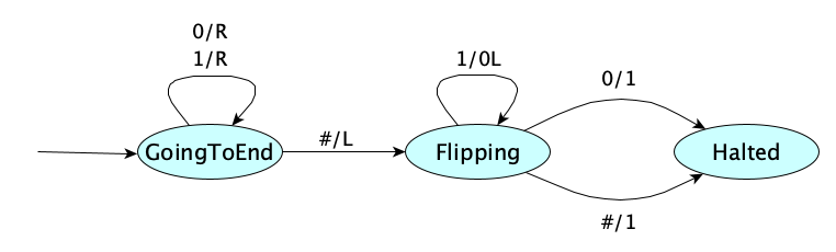
How many steps and extra memory cells does it take for different input sizes?

Input	Input Size	Time (steps)	Extra Space (tape cells)
0	1	1+1+0+1=3	1
1	1	1+1+1+1=4	1
00	2	2+1+0+1=4	1
01	2	2+1+1+1=5	1
10	2	2+1+0+1=4	1
11	2	2+1+2+1=6	1
000	3	3+1+0+1=5	1
001	3	3+1+1+1=6	1
010	3	3+1+0+1=5	1
011	3	3+1+0+3=7	1
100	3	3+1+0+1=5	1
101	3	3+1+1+1=6	1
110	3	3+1+0+1=5	1
111	3	3+1+3+1=8	1
0000	4	4+1+0+1=6	1
0001	4	4+1+1+1=7	1
...	...	...	...
1111	4	4+1+4+1=10	1
...	...	...	...

The most useful metric is the maximum number (worst-case) of steps or memory cells used for any input of a given size. In this case, for an input of size $n$, the most amount of work would be for the all-ones case:

• $n$ steps to scan just past the end
• 1 step to move back to the last bit
• $n$ flips
• 1 step to write the new 1-bit

We write $T(n) = 2n + 2$.

The best-case number of steps would be for the all-zeros case, namely $T(n) = n + 2$.

For this machine, space complexity $S(n) = 1$ since we need to store the blank symbol at the end of the input.

Here’s the single-tape Turing Machine for reversing a string (from the alphabet $\{a,b,c\}$):

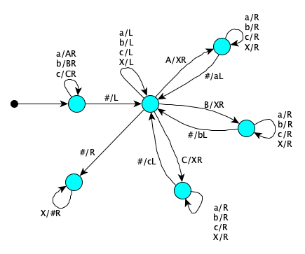
Let’s count steps for the input $abbacb$

⋅⋅abbacb⋅⋅⋅⋅⋅⋅⋅	Initial configuration
⋅⋅ABBACB⋅⋅⋅⋅⋅⋅⋅	6 steps to mark each symbol while moving right, 1 to go back to last symbol
⋅⋅ABBACXb⋅⋅⋅⋅⋅⋅	0 to find the B, 1 to X it, 0 to find where to put the b, 1 to write it
⋅⋅ABBAXXbc⋅⋅⋅⋅⋅	1 to find the C, 1 to X it, 2 to find where to put the c, 1 to write it
⋅⋅ABBXXXbca⋅⋅⋅⋅	3 to find the A, 1 to X it, 4 to find where to put the a, 1 to write it
⋅⋅ABXXXXbcab⋅⋅⋅	5 to find the B, 1 to X it, 6 to find where to put the b, 1 to write it
⋅⋅AXXXXXbcabb⋅⋅	7 to find the B, 1 to X it, 8 to find where to put the b, 1 to write it
⋅⋅XXXXXXbcabba⋅	9 to find the A, 1 to X it, 10 to find where to put the a, 1 to write it
⋅⋅⋅⋅⋅⋅⋅⋅bcabba⋅	11 to find the blank, 1 to move to the first X, 6 erases

This was a special case with $n=6$, but we can generalize to arbitrary $n$:

$$ (n+1) + \sum_{k=0}^{n-1}(4k+1) + 3n $$

which gives us $T(n) = 2n^2 + 3n + 1$. It’s quadratic.

Multiple Tapes

Now if we have a two-tape machine, reversal becomes much faster:

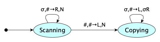
That’s $n$ steps to find the end, and $n$ steps to copy it to the second tape. $T(n) = 2n$.

Hey that went from quadratic to linear! The multitape model is often more realistic (think about real computers), so we can kind of assume it, though we really should always be explicit about the model we are using.

But is that cheating?

Not really. You can always be clear about your model.

But can we be loose with our models? Well, not too loose: each model needs to be finite (in terms of states or instructions), operate on finite inputs, and be made up of instructions that each take a finite amount of time. But if we do stick to reasonable models, a problem whose time complexity is a polynomial on one model will be polynomial on any other.

Being polynomially related turns out to matter. We’ll see why later.

In our case, linear and quadratic are both polynomial. We’re good.

Random Access

Random access models help us with problems that don’t always have to read the entire input, such as binary search.

We can use Random Access Turing Machines. or even register machines, but—and this is a really important but—we still have to count input in terms of bits, not in terms of unbounded-size registers. The number of bits is, after all, the true size of the input.

However, if the registers are bounded (e.g. 64 bits, 128 notes, etc.), then you can count registers rather than bits, because complexity measures will be within a constant factor, which in complexity theory, is just fine. It even lets you count bounded multiplication as a single instruction, which, as you might know, is technically quadratic time when the size of numbers are unbounded.

Nondeterminism

Remember that a nondeterministic Turing Machine accepts an input (answers YES) if there simply exists a computation path that leads to acceptance. How do we measure complexity on such a machine? We take the maximum number of steps or tape cells used on any accepting path. Irl, physical machines tend to be deterministic, and if so, will simulate nondeterministic machines via backtracking, so sure, we’d expect the time and space measurements to differ greatly between deterministic and nondeterministic machines. And they do.

Visualizing Nondeterminism

You can think of a nondeterministic machine as exploring all of its computation paths simultaneously, accepting if any path leads to a solution.

Real machines don’t work that way, but these models are theoretically very interesting: if you had a candidate solution, the nondeterministic machine would find it instantly. So nondeterministic machines model verification, while deterministic machines model the figuring out of a solution.

Probabilistic Machines

In a probabilistic machine, certain states are “coin flip” states, where the machine can transition to multiple possible next states with certain probabilities. The machine accepts an input if the probability of reaching an accepting state is above a certain threshold. Common thresholds are 1/2 or 2/3.

Parallel Machines

A parallel machine contains multiple sub-machines that run in parallel. At each “step,” each sub-machine performs a step of its own computation independently. Each sub-machine may or may not be running the same control program.

Start at this Wikipedia article to explore issues in analyzing parallel algorithms.

Boolean Circuit Computation Model

Rather than a Turing Machine, we can model a computation using Boolean circuits, that is, a directed acyclic graph where each node represents a gate (AND, OR, NOT). Complexity is based on the size of the circuit (number of gates), its depth (length of the longest path from an input to an output), and the fan-in (number of inputs to a gate).

Here’s an example of a circuit to add two 4-bit numbers, with size 17, depth 7, and fan-in 3:

Yes, this model is naturally parallel.

In practice, we are actually interested in families of Boolean circuits, where each input size has its own circuit.

Start your study at Wikipedia.

Quantum Machines

See Wikipedia’s articles on Quantum Turing Machines and Quantum circuits.

Interactive Proof Systems

Another Turing Machine alternative is the interactive proof system, an abstract machine in which two parties, a prover and a verifier, exchange messages to decide a language. Start at Wikipedia.

Input Encoding

Complexity measures can be sensitive to encoding.

To determine whether a signed binary number is negative, we need only one step to check the first bit, regardless of the input size: $T(n) = 1$. But to determine whether the number is even or odd, we have to scan the whole input to get to the end: $T(n) = n$.

But if we stored the number with the least significant bit first, then these complexities would be reversed. This is okay, since constant time and linear time are polynomially related.

What about encoding numbers in decimal rather than binary? This only speeds up computations by a factor of about $\log_2 10 \approx 3.32$. Constant factor speedups are not significant when studying inherent complexities, as you can imagine simply getting hardware which is $N$ times faster than your current machine. And again, we’re not measuring “absolute running time” but rather asymptotic behavior (growth rates as a function of input size).

Not all encodings are appropriate

One encoding that is not appropriate is unary. Unary encodings make the input exponentially larger than binary encodings, and make complexities look much smaller than they really are. The measures that differ between unary and binary encodings are not polynomially related.

Speaking of asymptotic behavior, it’s time to look at this topic formally.

Asymptotic Complexity

Measuring complexity in terms of the number of steps or memory cells as a function of input size is perfect for characterizing behaviors of computations. Such measurements are explicitly not concerned with absolute running times, because these vary with hardware, so it makes no sense to look at an abstract algorithm and ask for its exact running time. Even so, getting the exact time and space functions can be terribly tedious. The good news is that it is actually not necessary to get this precise! After all, what matters is the functions’ growth rates.

In fact, for complexity functions, we typically ignore:

• all but the “largest” (fastest growing) term, and
• any constant multipliers

So for example:

• $\lambda n . 0.4n^5 + 3n^3 + 253$ behaves asymptotically like $n^5$
• $\lambda n . 6.22 n \log n + \frac{n}{7}$ behaves asymptotically like $n \log n$

The justification for doing this is that:

• The difference between $6n$ and $3n$ isn’t meaningful when looking at algorithms abstractly, since getting a computer that is twice as fast makes the former behave exactly like the latter. The underlying speed of the computer never matters in abstract analysis. Only the algorithm structure itself matters.
• The difference between $2n$ and $2n+8$ is insignificant as $n$ gets larger and larger.
• If you are comparing the growth rates of, say, $\lambda n . n^3$ and $\lambda n . k n^2$, the former will always eventually overtake the latter no matter how big you make $k$. A leading constant can never make a function of a lower rank asymptotically worse than one from a higher rank.

How can we formalize this? That is, how do we formalize things like “the set of all quadratic functions” or the “set of all linear functions” or “the set of all logarithmic functions”? Paul Bachmann introduced a notation in 1894 that is still with us today.

Big-O: Asymptotic Upper Bounds

Definition Time! A function $f$ is in $O(g)$ whenever there exist constants $c$ and $N$ such that for every $n \ge N$, $f(n)$ is bounded above by a constant times $g(n)$. Formally:

$$ O(g) =_{\textrm{def}} \{ f \mid \exists c\!>\!0.\;\exists N\!\ge\!0.\;\forall n\!\ge\!N.\;0 \leq f(n) \leq c\cdot g(n) \} $$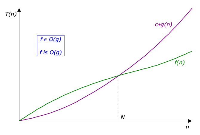

This means that $O(g)$ is the set of all functions for which $g$ is an asymptotic upper bound of $f$.

Examples:

• $\lambda n . 0.4 n^5 + 3n^3 + 253 \in O(\lambda n . n^5)$
• $\lambda n . 6.22n \log n + \frac{n}{7} \in O(\lambda n . n \log n)$

By convention, people usually drop the lambdas when writing expressions involving Big-O, so the above examples will actually appear in practice as:

• $O(n^5)$
• $O(n \log n)$

So in practice, we just throw away all the leading term then throw away its constant multiplier, but why is this justified? We’ll just provide an argument for a concrete case. (You can do the formal proof on your own.) Let’s show that $7n^4 + 2n^2 + n + 20 \in O(n^4)$. We have to choose $c$ and $N$. Let’s choose $c=30$ and $N=1$. So since $n \geq 1$:

$$ \begin{eqnarray} 7n^4 + 2n^2 + n + 20 & \leq & 7n^4 + 2n^4 + n^4 + 20n^4 \\ & \leq & (7 + 2 + 1 + 20) n^4 \\ & \leq & 30n^4 \end{eqnarray} $$

Too much technical detail? Want to review what this is all about? Here’s a video:

The Big-O Notation feels like we’re being sloppy and taking shortcuts. But it’s goal is to broadly classify certain algorithms, which has its use. Just don’t overuse though! Keep in mind that:

• Big-O notation is only useful for large $n$. The suppression of low-order terms and leading constants is misleading for small $n$. Be careful of functions such as:
  • $n^2 + 1000n$
  • $0.0001 n^5 + 10^6 n^2$
  • $10^{-4}2^n + 10^{5}n^3$
• Large constants may matter for small $n$. They signify overhead, which is common in algorithms that do a lot of initial setup to speed things up for large data sets. For example, when comparing $8n \log n$ and $0.01n^2$, the former is actually worse until $n$ gets up to $10,710$.
• You shouldn’t use Big-O to predict absolute running times. Robert Sedgewick has written: “[Big-O analysis] must be considered the very first step in a progressive process of refining the analysis of an algorithm to reveal more details about its properties.”
• Big-O is only an upperbound—it is not a tight upperbound. If an algorithm is in $O(n^2)$ it is also in $O(n^3)$, $O(n^{100})$, and $O(2^n)$. So it’s not really right to say that all complexity functions in $O(2^n)$ are terrible, because that set properly includes the set $O(1)$.

Big-Ω: Asymptotic Lower Bounds

There is a Big-$\Omega$ notation for lower bounds.

A function $f$ is in $\Omega(g)$ whenever there exist constants $c$ and $N$ such that for every $n \ge N$, $f(n)$ is bounded below by a constant times $g(n)$.

$$ \Omega(g) =_{\textrm{def}} \{ f \mid \exists c\!>\!0.\;\exists N\!\ge\!0.\;\forall n\!\ge\!N.\;0 \leq c \cdot g(n) \leq f(n) \} $$

Lower bounds are useful because they say that an algorithm requires at least so much time. For example, you can say that printing an array is $O(2^n)$ because $2^n$ really is an upper bound, it’s just not a very tight one! But saying printing an array is $\Omega(n)$ means it requires at least linear time which is more accurate.

Big-$\Theta$

When the lower and upper bounds are the same, we can use Big-Theta notation.

$$ \Theta(g) =_{\textrm{def}} \{ f \mid \exists c_1\!>\!0.\;\exists c_2\!>\!0.\;\exists N\!\ge\!0.\;\forall n\!\ge\!N.\;0 \leq c_1 \cdot g(n) \leq f(n) \leq c_2 \cdot g(n) \} $$

Example: printing each element of an array is $\Theta(n)$. Now that’s useful!

Most complexity functions that arise in practice are in Big-Theta of something. An example of a function that isn’t in Big-$\Theta$ of anything is $\lambda n . n^2 \cos n$.

Less-Common Complexity Functions

There are also little-oh and little-omega.

$$\omicron(g) =_{def} \{ f \mid \lim_{x\to\infty} \frac{f(x)}{g(x)} = 0 \}$$ $$\omega(g) =_{def} \{ f \mid \lim_{x\to\infty} \frac{f(x)}{g(x)} = \infty \}$$

There’s also the Soft-O:

$$\tilde{O}(g) =_{def} O(\lambda n.\,g(n) (\log{g(n)})^k)$$

Since a log of something to a power is bounded above by that something to a power, we have

$$\tilde{O}(g) \subseteq O(\lambda n.\,g(n)^{1+\varepsilon})$$

Comparison

For problems that appear in practice, the following are interesting and very general ways to classify.

Kind	$O(\lambda\,n. \ldots)$	Description
Constant	$1$	Fixed number of steps or memory cells, regardless of input size
Logarithmic	$\log n$	Number of steps or memory cells proportional to log of input size
Polynomial	$n^k$, $k \geq 1$	Number of steps or memory cells a polynomial of input size
Exponential	$c^n$, $c > 1$	Number of steps or memory cells exponential of input size

We can introduce more! Expressed as times, we have:

Kind	$O(\lambda\,n. \ldots)$	Examples
Constant	$1$	Retrieving the first element in a list
Inverse Ackermann	$\alpha(n)$
Iterated Log	$\log^{*} n$
Loglogarithmic	$\log \log n$
Logarithmic	$\log n$	Binary Search
Polylogarithmic	$(\log n)^c$, $c>1$
Fractional Power	$n^c$, $0<c<1$
Linear	$n$	Max or min of an unsorted array
N-log-star-n	$n \log^{*} n$	Seidel’s polygon triangulation algorithm
Linearithmic	$n \log n$	Mergesort, Fast Fourier Transform
Quadratic	$n^2$	Insertion Sort
Cubic	$n^3$
Polynomial	$n^c$, $c\geq 1$
Quasipolynomial	$n^{\log n}$
Subexponential	$2^{n^\varepsilon}$, $0<\varepsilon<1$
Exponential	$c^n$, $c>1$	Brute-force Matrix Chain Multiplication
Factorial	$n!$	Brute-force Traveling Salesperson
N-to-the-n	$n^n$
Double Exponential	$2^{2^{cn}}$	Deciding Presburger Arithmetic formulas
Ackermann	$A(n)$
Unbounded Time	$\infty$	Busy Beaver

For fun, let’s connect these functions to clock time. If we had a machine that could do one million operations per second, here’s how long it would take to carry out computations of size $n$ for different time complexity functions.

$T(n)$	10	20	50	100	1000	1000000
1	1 μs	1 μs	1 μs	1 μs	1 μs	1 μs
$\log n$	3.322 μs	4.322 μs	5.644 μs	6.644 μs	9.966 μs	19.93 μs
$n$	10 μs	20 μs	50 μs	100 μs	1 ms	1 second
$n \log n$	33.22 μs	86.44 μs	282.2 μs	664.4 μs	9.966 ms	19.93 seconds
$n^2$	100 μs	400 μs	2.5 ms	10 ms	1 second	11.57 days
$1000 n^2$	100 ms	400 ms	2.5 seconds	10 seconds	16.67 minutes	31.688 years
$n^3$	1 ms	8 ms	125 ms	1 second	16.67 minutes	31,688 years
$n^{\log n}$	2.099 ms	419.7 ms	1.078 hours	224.5 days	2.502×1016 years	1.231×10106 years
$1.01^n$	1.105 μs	1.220 μs	1.645 μs	2.705 μs	20.96 ms	7.493×104307 years
$0.000001 \times 2^n$	1.024 ns	1.049 μs	18.76 minutes	4.017×1010 years	3.395×10281 years	3.137×10301010 years
$2^n$	1.024 ms	1.049 seconds	35.68 years	4.017×1016 years	3.395×10287 years	3.137×10301016 years
$n!$	3.629 seconds	77,093 years	9.638×1050 years	2.957×10144 years	1.275×102554 years	2.619×105565695 years
$n^n$	2.778 hours	3.323×1012 years	2.814×1071 years	3.169×10186 years	3.169×102986 years	3.169×105999986 years
$2^{2^n}$	5.697×10294 years	2.136×10315639 years	103.389×1014 years	103.382×1029 years	103.323×10300 years	102.980×10301029 years

Exponents are hard to wrap your head around. The earth formed about $4.5 \times 10^9$ years ago and the big bang occurred about $13.8 \times 10^9$ years ago (so say our best estimates to date). So you’re not going to see $2^{100}$ operations performed on a single computer in your lifetime. Even if it could do a trillion operations per second, you’d still need 2.9 universe lifetimes. And 100 is a pretty small $n$. 🤯

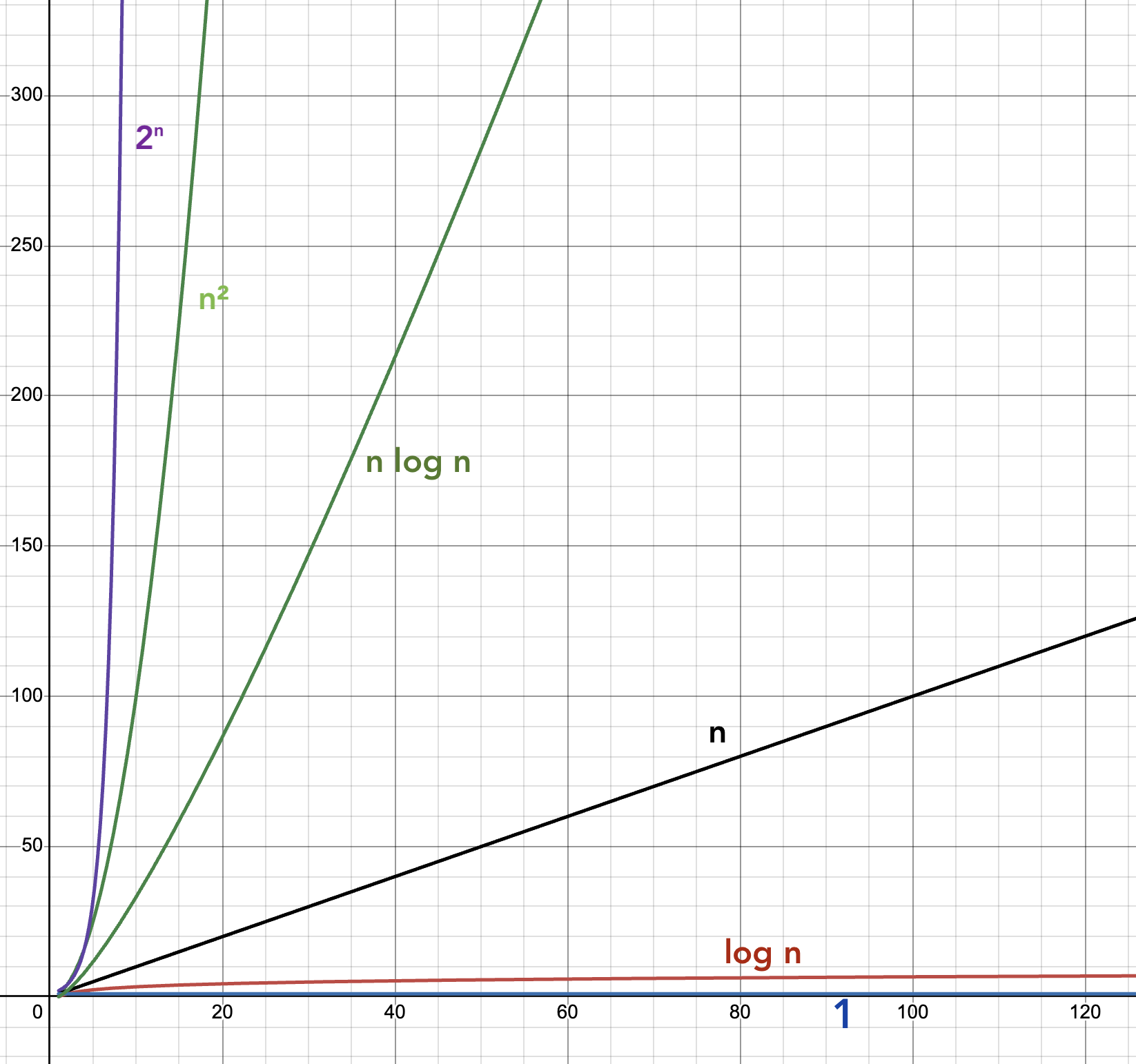
If we use a log-scale on the vertical axis, we can start to see something important:

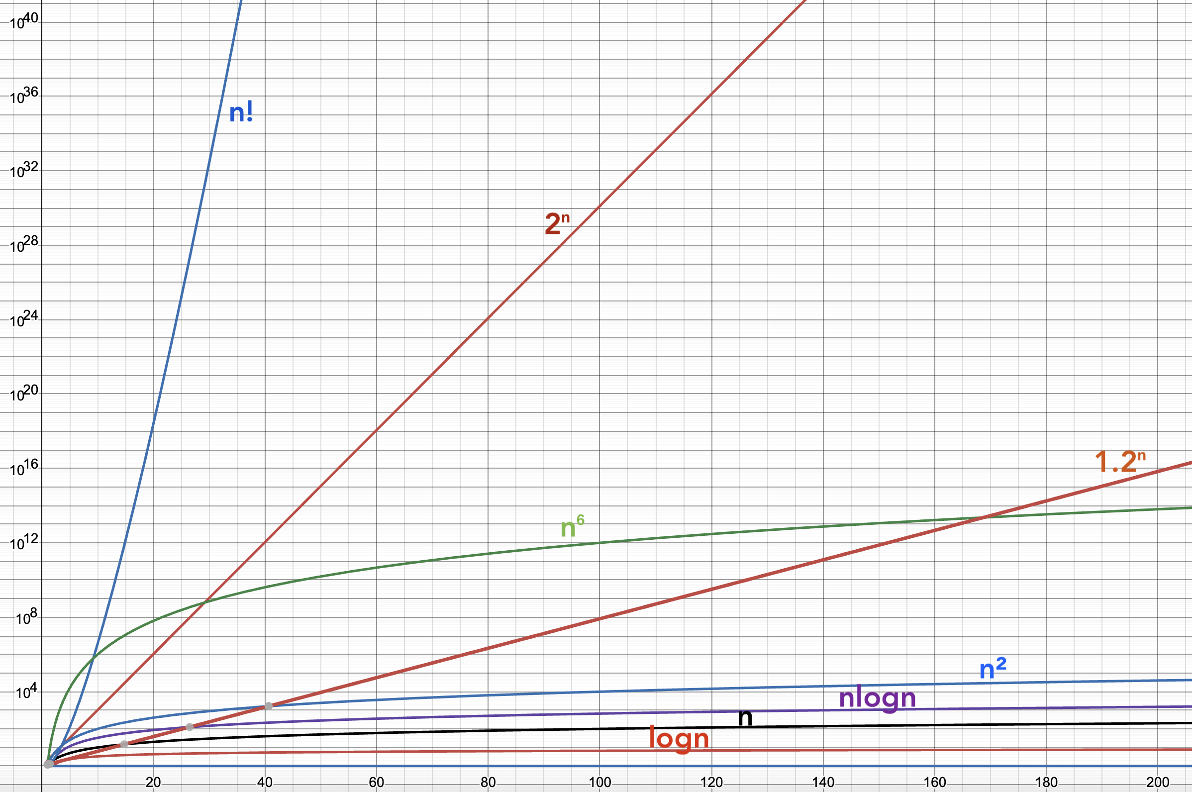
Anything polynomial, even with a high degree, starts to look flatter (grows slower) as $n$ gets really large. But exponentials, even with smallish bases (but strictly greater than 1), will eventually blow away every polynomial. Every. Single. One.

More on these big numbers

Maybe you are not too impressed with exponents in the thousands? Consider this: the volume of the observable universe, as far as we can tell, is about $3.57 \times 10^{80}$ cubic meters, which means the approximate number of Planck volumes it contains is around $10^{186}$. That’s nothing compared to some of the numbers in this chart.

The divide between the polynomial and the exponential is so noticeable that it just seems to be something fundamental to the universe. Polynomial time algorithms are called easy or tractable, exponential and beyond are hard or intractable. Because this is such a noticeable division, we (in theory-land) allow ourselves flexibility in computational models, as long as they don’t move complexities between the polynomial and the exponential.

We can vary models as long as they are polynomially related.

Complexity Classes

We can often simplify the kinds of statements we make about complexity by recasting question of “how many steps (or how much memory) it takes to compute an answer” into “how many steps (or how much memory) does it take to decide membership in a language?” This means we can group languages into classes, much like we did in computability theory. For example, the problem of finding the shortest path between two vertices in a graph, phrased as an optimization problem is:

$$\textrm{Given graph $G$ and vertices $s$ and $t$, what is the length of the shortest path in $G$ from $s$ to $t$?}$$

This can be recast as a decision problem:

$$\textrm{Is there a path in $G$ from $s$ to $t$ of length at most $k$?}$$

Then as a language acceptance problem:

$$\{ \langle G, s, t, k \rangle \mid \textrm{$\exists$ a path in $G$ from $s$ to $t$ of length at most $k$} \}$$

The for major generic language classes are, where $f$ is a proper complexity function of type $\mathbb{N} \to \mathbb{N}$:

Class	Description
$\textsf{DTIME}(f)$	Decidable by a deterministic machine in time $O(f)$
$\textsf{DSPACE}(f)$	Decidable by a deterministic machine in space $O(f)$
$\textsf{NTIME}(f)$	Decidable by a non-deterministic machine in time $O(f)$
$\textsf{NSPACE}(f)$	Decidable by a non-deterministic machine in space $O(f)$

Now let’s get more specific. There are hundreds of complexity classes, but a handful are pretty important. Here are the most basic ones to know:

Class	Description
$\textsf{P}$	Languages decidable by a deterministic machine in polynomial time. Could also be called $\textsf{PTIME}$ but no one says that. Formally, it is $$\textsf{P} = \bigcup_{k \in \mathbb{N}} \textsf{DTIME}(n^k)$$
$\textsf{NP}$	Languages decidable by a non-deterministic machine in polynomial time. Formally, $$\textsf{NP} = \bigcup_{k \in \mathbb{N}} \textsf{NTIME}(n^k)$$ Although defined in terms of nondeterministic machines, a corollary is a more useful way to think of this class: $\textsf{NP}$ is the set of all decision problems for which a YES answer can be verified in polynomial time by a deterministic machine
$\textsf{PSPACE}$	Deterministic polynomial space
$\textsf{NPSPACE}$	Nondeterministic polynomial space
$\textsf{EXP}$	Deterministic exponential time (sometimes called $\textsf{EXPTIME}$). Formally, $$\textsf{EXP}=\bigcup_{k \in \mathbb{N}} \textsf{DTIME}(2^{n^k})$$
$\textsf{NEXP}$	Nondeterministic exponential time (sometimes called $\textsf{NEXPTIME}$)
$\textsf{EXPSPACE}$	Deterministic exponential space
$\textsf{NEXPSPACE}$	Nondeterministic exponential space
$\textsf{L}$	Deterministic logarithmic space (can be called $\textsf{LOGSPACE}$). Formal definition is simply $$\textsf{L} = \textsf{DSPACE}(\log n)$$
$\textsf{NL}$	Nondeterministic logarithmic space (can be called $\textsf{NLOGSPACE}$)

Researchers have come up with various theorems, such as the time hierarchy theorem and the space hierarchy theorem, which lead us to some set containment hierarchies. We know some things:

• $\textsf{PSPACE} = \textsf{NPSPACE}$
• $\textsf{EXPSPACE} = \textsf{NEXPSPACE}$
• $\textsf{L} \subseteq \textsf{NL} \subseteq \textsf{P} \subseteq \textsf{NP} \subseteq \textsf{PSPACE} \subseteq \textsf{EXP} \subseteq \textsf{NEXP} \subseteq \textsf{EXPSPACE}$

But get this: we actually don’t know which of these containments are proper!

• Is $\textsf{L} = \textsf{NL}$? We don’t know.
• Is $\textsf{NL} = \textsf{P}$? We don’t know.
• Is $\textsf{P} = \textsf{NP}$? We don’t know.
• Is $\textsf{NP} = \textsf{PSPACE}$? We don’t know.
• Is $\textsf{PSPACE} = \textsf{EXP}$? We don’t know.
• Is $\textsf{EXP} = \textsf{NEXP}$? We don’t know.
• Is $\textsf{NEXP} = \textsf{EXPSPACE}$? We don’t know.

But we do know some of the big steps!

• $\textsf{P} \subsetneq \textsf{EXP}$ (by the time hierarchy theorem)
• $\textsf{L} \subsetneq \textsf{PSPACE} \subsetneq \textsf{EXPSPACE}$ (by the space hierarchy theorem)

Those 10 complexity classes are the ones you absolutely need to know. Next, learn the ones in the following diagram.

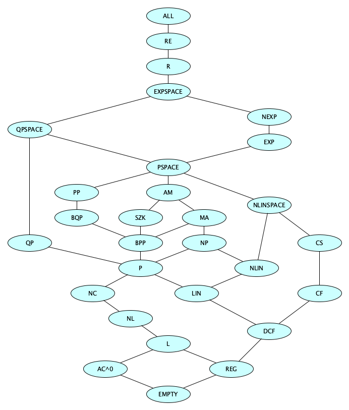
Here’s a run-down on the classes in this diagram, with some of the descriptions horribly oversimplified.

Class	Description
$\textsf{EMPTY}$	The empty class (contains no languages)
$\textsf{REG}$	Regular languages (decided by FAs)
$\textsf{DCFL}$	Deterministic context-free languages (decided by DPDAs)
$\textsf{CFL}$	Context-free languages (decided by PDAs)
$\textsf{CSL}$	Context-sensitive languages (decided by LBAs)
$\textsf{R}$	Recursive languages (decided by Turing machines that always halt)
$\textsf{RE}$	Recursively enumerable languages (recognized by Turing machines)
$\textsf{ALL}$	All languages
$\textsf{LIN}$	Linear Time
$\textsf{NLIN}$	Nondeterministic Linear Time
$\textsf{P}$	Polynomial Time
$\textsf{NP}$	Nondeterministic Polynomial Time
$\textsf{QP}$	Quasipolynomial Time
$\textsf{EXP}$	Exponential Time
$\textsf{NEXP}$	Nondeterministic Exponential Time
$\textsf{L}$	Logarithmic Space
$\textsf{NL}$	Nondeterministic Logarithmic Space
$\textsf{QPSPACE}$	Quasipolynomial Space
$\textsf{PSPACE}$	Polynomial Space (determinism does not matter)
$\textsf{EXPSPACE}$	Exponential Space (determinism does not matter)
$\textsf{AC}^0$	Solvable by constant-depth, polynomial-size circuits with unbounded fan-in
$\textsf{NC}$	Solvable by uniformly-generated with polynomially-size circuits with polylogarithmically-bounded depth and fan-in 2
$\textsf{P/poly}$	Solvable by nonuniform polynomial-size circuits
$\textsf{SZK}$	Verifiable by a statistical zero-knowledge proof protocol
$\textsf{MA}$	Verifiable by Merlin-Arthur protocol
$\textsf{AM}$	Verifiable by Arthur-Merlin protocol
$\textsf{QMA}$	Verifiable by Quantum Merlin-Arthur protocol
$\textsf{BPP}$	Bounded-error Probabilistic Polynomial: Solvable by $\textsf{NP}$ machines that for YES instances, at least 2/3 of the computation paths accept and for NO instances, at least 2/3 reject
$\textsf{PP}$	Probabilistic Polynomial: Solvable by $\textsf{NP}$ machines that for YES instances, at least 1/2 of the computation paths accept and for NO instances, at least 1/2 reject
$\textsf{RP}$	Randomized Polynomial: Solvable by $\textsf{NP}$ machines that for YES instances, at least 1/2 of the computation paths accept and for NO instances, all reject
$\textsf{ZPP}$	Zero-error Probabilistic Polynomial: Solvable by probabilistic TMs in expected polynomial time with zero error. Formally defined as $\textsf{RP} \cap \textsf{co-RP}$
$\textsf{BQP}$	Bounded-error Quantum Polynomial: Solvable by a quantum TM in polynomial time with at most 1/3 probability of error

The Complexity Zoo

We have barely begun.

But that’s okay—these notes are meant only to be an introduction.

The Complexity Zoo is an extensive online resource cataloging complexity classes. As of December 2025, there are 551 language classes documented.

Go take a tour. Begin with the Petting Zoo.

By all means do not miss Satoshi Hada's Complexity Zoo Browser.

Gabe Robins has done a nice little annotation on the big diagram from the Zoo. It’s very near the bottom of his notes on resource bounded computation. He’s highlighted the major complexity classes as well as the ones we saw when studying automata theory. Worth a look!

There’s a super cool interactive active inclusion diagram. Check it out!

If at any time you just want to scan a brief list of classes, without diving into details at all, getting some big ideas and nothing more, Wikipedia has just such a list.

Hardness and Completeness

Remember that the harder a problem is, the more resources it requires to solve. In any class of problems, it makes sense to talk about the “hardest” problems in the class. We can define this notion formally!

The reduction used has to be in a class that is considered efficient for the context, typically polynomial time for anything in $\textsf{NP}$ or above. In general, the reduction has to be in a strictly smaller class than the class being considered.

P and NP

We have to go deeper into these two classes. There is so, so much to say. Many nontechnical people have heard of the P vs NP Question. Here are some facts:

• $\textsf{P}$ is (roughly) the class of problems that we can solve efficiently.
• $\textsf{NP}$ is (roughly) the class of problems for which we can verify solutions efficiently.
• Zillions (not exaggerating) of useful problems are known to be $\textsf{NP}$-hard or $\textsf{NP}$-complete.
• We don’t know if $\textsf{P} = \textsf{NP}$, but we suspect $\textsf{P} \neq \textsf{NP}$.
• Thousands of people have been trying for at least half a century to resolve this question, but no one has succeeded yet.
• Finding a solution to this problem is incredibly challenging and may require the invention of new branches of mathematics to solve.
• There is a million-dollar prize waiting for anyone who can resolve the P vs NP question.
• If $\textsf{P} = \textsf{NP}$ under a certain condition, the world would be a radically different place (more on this below).

An example of an $\textsf{NP}$-hard problem is Sudoku: easy to verify but hard to solve.

There are some good videos out there to give you a sense of this problem. This is a well-known video which is kind of a classic, and you should watch it first:

A newer one that introduces the idea that the P vs. NP question is really about algorithm inversion:

Jade’s P vs. NP video was seen previously in the notes on Theories of Computation. She has a sequel focused on NP-completeness:

Examples of NP-Complete Problems

The readings and videos above will introduce you to the history of NP-completeness and provide examples of NP-complete problems. The list of known and useful NP-complete problems is stunningly large. It is fascinating that they are all in some sense all versions of the same problem. Here’s a tiny fraction of that list:

• Satisfiability
• Traveling Salesperson
• Knapsack
• Job Scheduling
• Vehicle Routing
• Integer Programming
• Multi-commodity Flow
• k-Means
• Neural Net Training
• SVM Training
• Protein Folding
• Multiple Sequence Alignment
• Graph Coloring
• Hamiltonian Cycle
• Vertex Cover
• Max Cut
• Max Clique
• Graph Coloring
• Subset Sum
• 3-SAT
• Tetris
• Candy Crush
• Minesweeper

Known Polynomial-Time Friends

Here’s something interesting. A lot of NP Problems have special cases on their inputs for which a solution is known to ne in $\textsf{P}$.

NP-Complete or NP-Hard Problem	Restrictions Known to Be in P
SAT	All clauses have at most 2 literals, or all clauses are Horn clauses
Graph Coloring	2-Coloring
Hamilton Cycle	Dense Graphs
Vertex Cover	Bipartite Graphs, Trees
Traveling Salesperson	Trees, Graphs with max degree 2
Clique	Planar graphs, chordal graphs

Sometimes there is a mirror problem that is in P.

NP-Complete or NP-Hard Problem	Variants Known to Be in P
Hamilton Cycle	Euler Tour
Vertex Cover	Edge Cover
Independent Set	Maximum Matching
Integer Linear Programming	Linear Programming
Longest Path	Shortest Path
Max Cut	Min Cut
Min Flow	Max Flow

Why is this interesting?

The difference between problems known to be in $\textsf{P}$ and those in $\textsf{NP}$ but not known to be in $\textsf{P}$ is sometimes very subtle. You should know how to tell the difference. You may have to design an algorithm for something. Knowing whether it is known-$\textsf{P}$ or not might matter a lot! So it’s a good idea to study a number of existing problems and know why they are in $\textsf{P}$, or prove them to be $\textsf{NP}$-complete. Or maybe show that they are neither.

Proving $\textsf{P} = \textsf{NP}$ or $\textsf{P} \neq \textsf{NP}$

Do you want that million-dollar prize? Here’s how you can get it:

• If you can show just one $\textsf{NP}$-complete problem is in $\textsf{P}$, then this proves $\textsf{P} = \textsf{NP}$.
• If you can show just one $\textsf{NP}$-complete problem is not in $\textsf{P}$, then this proves $\textsf{P} \neq \textsf{NP}$.

But many thousands of brilliant people have tried to solve this problem. We still don’t have an answer. But we do know that answering this question won’t be easy. Proving this either way is a massive challenge! For example, to prove $\textsf{P} \neq \textsf{NP}$, the usual mathematical techniques just don’t work. There are “barriers” that show these techniques are impossible: the relativization barrier, the natural proofs barrier, and the algebrization barrier.

Some people think we will have to use something like Geometric Complexity Theory (which very few people understand), or to invent entirely new branches of mathematics to make progress on this problem.

Don’t let that stop you from trying. But be careful:

In 1976 when I was a graduate student in Germany, I bumped into a new professor who had been a particularly bright student .... He had been given a full professorship ... pretty much right after receiving his Doctorate. He told me straight out that he was going to solve the P=NP problem. He exuded confidence in his abilities and fairly gloated over the fact that he had a leg up on his American counterparts, because, as a German professor, he could pretty much dictate his own schedule. That is, he could go into his room, lock his door, and focus on The Problem.

Many years later I asked about this person, and I got answers indicating that no one really knew anything about him. He was still a professor as far as anyone could tell, but he had turned into a recluse and a virtual hermit, which seemed to baffle everyone.

— Rocky Ross

What if $\textsf{P} = \textsf{NP}$?

Although nearly 90% of experts believe $\textsf{P} \neq \textsf{NP}$, we don’t really know for sure, and it’s fun to entertain the possibility that $\textsf{P} = \textsf{NP}$. If the classes are equal, then one or two things are the case:

• The polynomial-time algorithms for $\textsf{NP}$-complete problems are galactic, perhaps $\Omega(n^{10^{100}})$, which even for values of $n$ into the gazillions is way worse that than brute-forcing all $2^n$ candidate solutions. In this case, nothing changes. The interesting $\textsf{NP}$-complete problems remain intractable.
• The polynomial-time algorithms have practical lower bounds, perhaps $\Omega(n^4)$, in which case the world would be radically different:
  • TSP is efficiently solvable, so we routing and scheduling can be done with perfect supply chains and zero waste. This includes allocation compute resources in data centers, not just trucks and planes.
  • Protein folding is efficiently solvable, so we can design drugs instantly, enabling us to cure cancer and mass-produce plastic-eating enzymes.
  • Circuit layout is efficiently solvable, so we can design optimal circuits with perfect space and power efficiency.
  • Optimal inference is efficiently solvable, so neural networks can be trained perfectly and instantly.
  • Integer factorization is efficiently solvable, so cryptography as we know it (RSA, Diffie-Hellman, ECC, AES, SHA) would be broken, requiring a shift to one-time pads (impractical for everyone), quantum-resistant cryptography (possibly expensive), more steganography (risky), or the invention of new cryptographic methods (ooooh, there’s a research topic for you).

Dealing with $\textsf{NP}$-completeness today

Since we don’t know whether $\textsf{P} = \textsf{NP}$, we just don’t have any general efficient solutions to $\textsf{NP}$-complete problems. We have some options:

• Write an implementation using intelligent backtracking. This will solve the problem exactly but there will be inputs for which the run time is still longer than your lifetime.
• Write something that looks for special input cases and solves them specially, e.g. for SUBSET SUM having all positive inputs and a relatively small value of $k$, there’s a pretty fast dynamic programming solution.
• Write an implementation using randomization or heuristics, that runs quickly but fails to give a correct answer a certain small percentage of the time.
• For optimization problems, write something that runs quickly and gives an answer that is not optimal, but not too far from optimal (an approximation algorithm).

We’d use the same strategies after $\textsf{P} \neq \textsf{NP}$ is proven, or after $\textsf{P} = \textsf{NP}$ is proven but with a galactic lower bound.

Further Reading

There is no way to list all of the P vs NP resources out there, but here are a few notable ones:

• The P versus NP Page (seems to have not been updated since 2016)
• A Brief Summary of the P vs. NP Problem from MIT News
• Wikipedia: P vs NP Problem, List of NP Complete Problems
• NP-Completeness on xkcd: TSP, Restaurant Orders.
• David Johnson’s A Brief History of NP-Completeness, 1954–2012
• Blog posts and papers by Scott Aaronson: Ten Reasons to Believe P ≠ NP, Is P=NP Independent of ZFC?, NP-Complete Problems and Physical Reality

Open Problems

Here’s a closing observation that shows why complexity theory is fun.

Some of the most interesting open problems—that is, problems for which the answer is “we don’t know”—in computer science are related to complexity theory.

See Wikipedia’s List of Unsolved Problems in Computer Science.

Recall Practice

Here are some questions useful for your spaced repetition learning. Many of the answers are not found on this page. Some will have popped up in lecture. Others will require you to do your own research.

1. How are computability and complexity related and how are they different?
   Computability theory is concerned with whether a problem can be solved at all, while complexity theory is concerned with how efficiently a problem can be solved.
2. What are the primary measures of complexity?
   Time and space.
3. What are the three main computational models used in complexity theory?
   Turing machines, Boolean circuit families, and interactive proofs.
4. What are some variations on computational models?
   Nondeterminism, Randomness, Quantum computation.
5. How is time measured on a Turing Machine?
   As a function from the input size to the number of steps the machine takes.
6. How is space measured on a Turing Machine?
   As a function from the input size to the number of tape cells the machine uses, not including the space for the input.
7. What are the traditional names of the time complexity and space complexity functions?
   $T(n)$ for time complexity and $S(n)$ for space complexity, where $n$ is the input size.
8. How does the time complexity differ for the string reversal problem on single vs. multiple tape machines?
   Quadratic on a single-tape machine and linear on a multi-tape machine.
9. What technique is often used to simulate nondeterminism on a deterministic machine?
   Backtracking.
10. How does a probabilistic machine differ from a nondeterministic machine?
    A probabilistic machine uses random choices to influence its computation, while a nondeterministic machine essentially explores all computation paths simultaneously.
11. What aspects of a Boolean Circuit affect its complexity?
    The size (number of gates), depth (longest path from input to output), and fan-in (number of inputs to a gate) of the circuit.
12. What is an interactive proof system?
    A computational model where a verifier interacts with a prover to determine the validity of a statement, which, is equivalent to deciding a language.
13. Why do we have to be careful with input encoding when measuring complexity?
    If inputs are encoded inefficiently, we get misleading complexity measurements.
14. What is an example of an inefficient input encoding that is verboten?
    Unary encoding for numbers.
15. What is meant by asymptotic complexity?
    The behavior of a function as the input size grows towards infinity.
16. Why are we interested in asymptotic complexity?
    Measuring the exact time can be complex and not so relevant in practice because different computers run at different speeds.
17. How do we get an asymptotic measure?
    Keep the dominant terms and ignore constant factors.
18. What is Big-O all about?
    Asymptotic upper bounds.
19. Why must Big-O notation be used carefully? Try to give three reasons.
    (1) it is only an upper bound, not a tight upper bound, (2) it ignores constant factors and lower-order terms that may matter a great deal for small $n$, (3) it has nothing to do with absolute running times.
20. What is the formal definition of the set $O(g)$?
    $ O(g) =_{\textrm{def}} \{ f \mid \exists c\!>\!0.\;\exists N\!\ge\!0.\;\forall n\!\ge\!N.\;0 \leq f(n) \leq c\cdot g(n) \} $
21. What is Big-$\Omega$ all about?
    Asymptotic lower bounds.
22. What is the formal definition of the set $\Omega(g)$?
    $ \Omega(g) =_{\textrm{def}} \{ f \mid \exists c\!>\!0.\;\exists N\!\ge\!0.\;\forall n\!\ge\!N.\;0 \leq c\cdot g(n) \leq f(n) \} $
23. What is Big-$\Theta$ all about?
    Asymptotic tight bounds.
24. What is the formal definition of the set $\Theta(g)$?
    $ \Theta(g) =_{\textrm{def}} O(g) \cap \Omega(g) $
25. What kind of functions are not in Big-$\Theta$ of anything and why don’t we see them often?
    Functions that oscillate too wildly, such as $\lambda n . n^2 \cos n$. We rarely encounter them because most reasonable time and space complexity functions increase as $n$ increases.
26. What are trivial examples of constant, logarithmic, linear, linearithmic, polynomial, quasipolynomial, and exponential time complexities?
    Constant: $1$, Logarithmic: $\log n$, Linear: $n$, Linearithmic: $n \log n$, Polynomial: $n^2$, Quasipolynomial: $n^{\log n}$, Exponential: $2^n$.
27. What kind of terms are used to refer to Polynomial-time vs. non-polynomial-time problems?
    Tractable vs. intractable, or easy vs. hard.
28. What can be said about polynomial-time algorithms with very high degree?
    They are efficient only for small input sizes.
29. What is a complexity class?
    A set of languages (or decision problems) that share a common resource-based complexity, such as time or space.
30. What are the four most well-known generic language classes?
    $\textsf{DTIME}(f)$, $\textsf{DSPACE}(f)$, $\textsf{NTIME}(f)$, $\textsf{NSPACE}(f)$.
31. How is $\textsf{DTIME}(f)$ defined?
    The class of languages decidable by a deterministic Turing machine in $O(f(n))$ time.
32. Arrange the following in subset order: $\textsf{NP}$, $\textsf{L}$, $\textsf{PSPACE}$, $\textsf{NEXPSPACE}$, $\textsf{P}$, $\textsf{EXP}$, $\textsf{NEXP}$, $\textsf{NPSPACE}$, $\textsf{NL}$, $\textsf{EXPSPACE}$.
    $\textsf{L} \subseteq \textsf{NL} \subseteq \textsf{P} \subseteq \textsf{NP} \subseteq \textsf{PSPACE} = \textsf{NPSPACE} \subseteq \textsf{EXP} \subseteq \textsf{NEXP} \subseteq \textsf{EXPSPACE} = \textsf{NEXPSPACE}$.
33. Why is $\textsf{REG} \subseteq \textsf{L}$?
    Because regular languages can be decided by a deterministic finite automaton, which uses constant space, and constant space is a subset of logarithmic space.
34. Why is $\textsf{CS} \subseteq \textsf{NLINSPACE}$?
    Because context-sensitive languages can be decided by a linear bounded automaton, which uses linear space.
35. Why is $\textsf{P} \subseteq \textsf{QP}$?
    Because polynomial-time algorithms are a subset of quasi-polynomial-time algorithms.
36. What are examples of complexity classes for which circuits are the primary model of computation?
    $\textsf{AC}^0$, $\textsf{NC}$, and $\textsf{P/poly}$.
37. What are examples of complexity classes for which interactive proofs are the primary model of computation?
    $\textsf{SZK}$, $\textsf{MA}$, $\textsf{AM}$, and $\textsf{QMA}$.
38. What are examples of complexity classes for which probabilistic machines are the primary model of computation?
    $\textsf{BPP}$, $\textsf{RP}$, $\textsf{ZPP}$, and $\textsf{PP}$.
39. What are examples of complexity classes for which quantum machines are the primary model of computation?
    $\textsf{BQP}$ and $\textsf{QMA}$.
40. Who is the Zookeeper of the Complexity Zoo?
    Scott Aaronson.
41. What does it mean for a problem to be hard for a complexity class?
    Every problem in the class can be reduced to it using a suitable reduction.
42. What does it mean for a problem to be complete for a complexity class?
    It is in the class and every problem in the class can be reduced to it using a suitable reduction.
43. What is the colloquial way to define $\textsf{P}$ and $\textsf{NP}$?
    $\textsf{P}$ is the class of problems that can be solved in polynomial time; $\textsf{NP}$ is the class of problems for which a solution can be verified in polynomial time.
44. Does $\textsf{P} = \textsf{NP}$?
    We don’t know. This is one of the most important open questions in computer science.
45. Who will give you a million dollars if you prove $\textsf{P} = \textsf{NP}$ or $\textsf{P} \neq \textsf{NP}$?
    The Clay Mathematics Institute, as part of their Millennium Prize Problems.
46. Which of the following $\textsf{NP}$ problems—VERTEX COVER, 2-SAT, HAMILTON CYCLE, EULER TOUR, CLIQUE, MINIMUM SPANNING TREE, SHORTEST PATH—are not known to be in $\textsf{P}$?
    VERTEX COVER, HAMILTON CYCLE, and CLIQUE are not known to be in $\textsf{P}$.
47. Under what conditions would a proof of $\textsf{P} = \textsf{NP}$ not change the world much?
    If the polynomial-time algorithms for $\textsf{NP}$-complete problems are galactic or if the proof says we know polynomial-time algorithms exist but doesn't provide a practical way to find them.
48. What are examples of world-changing effects that would occur if $\textsf{P} = \textsf{NP}$ with a feasible lower bound?
    The usual cryptograph methods would be broken, routing and transportation would become optimzed, better drugs would be created efficiently.
49. What techniques are used today to deal with intractable problems?
    Heuristics, finding special cases, avoiding large inputs, randomization, approximations.

Summary