Mathematics for Computation
Wait What is Math?
You’re not going to find an official definition of mathematics that everyone will agree on, but many people would be okay with saying that it involves reasoning about quantity, change, structure, chance, causality, and space aided by the discovery of abstract patterns and the invention of models.
Math aims to help us both (1) explain real-world phenomena and (2) discover truths that transcend the physical world. It’s such a well-known human activity that Wikipedia has an article on it! Seriously! Who knew?
Where does it come from?
No one knows for sure, but there’s a great book on the topic that just might have the answer. If you look at the evolution of life and consciousness you might get some ideas. The earliest life forms may have only survived by bumping into food. Natural selection led to sensing abilities enabling organisms to move toward the food. Next, lifeforms capable of making “models of their surroundings” so they could both navigate around obstacles and remember where the food was gained an evolutionary advantage.
Was it invented or discovered?
This question has been asked millions of times. Seriously.
The answer is probably both!
The question is so popular we can even question the question:
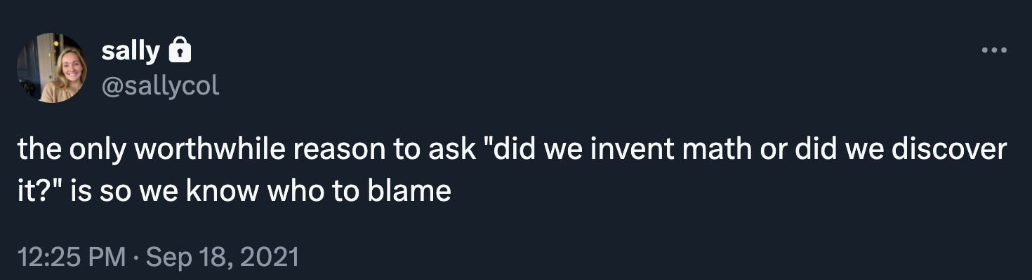
Whatever your take on this question is, Math has proven to be unreasonably effective in the natural sciences.
What are some of its branches?
Math is a big field of study. Here’s how Wikipedia breaks it down (others may have different takes):
| Branch | Topics |
|---|---|
| Foundations | Philosophy of Mathematics • Mathematical Logic • Information Theory • Set Theory • Type Theory • Category Theory |
| Algebra | Abstract • Boolean • Clifford • Commutative • Elementary • Field Theory • Group Theory • Homological • Lie • Linear • Multilinear • Ring Theory • Universal |
| Analysis | Calculus • Real Analysis • Complex Analysis • Hypercomplex Analysis • Differential Equations • Functional Analysis • Harmonic Analysis • Measure Theory |
| Discrete | Combinatorics • Discrete Geometry • Graph Theory • Matroid Theory • Order Theory |
| Geometry | Algebraic • Affine • Analytic • Arithmetic • Complex • Computational • Convex • Differential • Discrete • Euclidean • Finite • Information • Projective |
| Number Theory | Algebraic • Analytic • Arithmetic • Diophantine Geometry |
| Topology | General • Algebraic • Differential • Geometric • Homotopy Theory • Knot Theory |
| Applied | Control theory • Operations Research • Probability • Statistics • Game Theory |
| Computational | Computer Science • Theory of Computation • Computational Complexity • Numerical Analysis • Optimization • Computer Algebra |
Another organization of topics can be found at Quanta Magazine’s Map of Mathematics. There’s also a cool Map of Mathematics video by Dominic Walliman, from which this poster can be found:
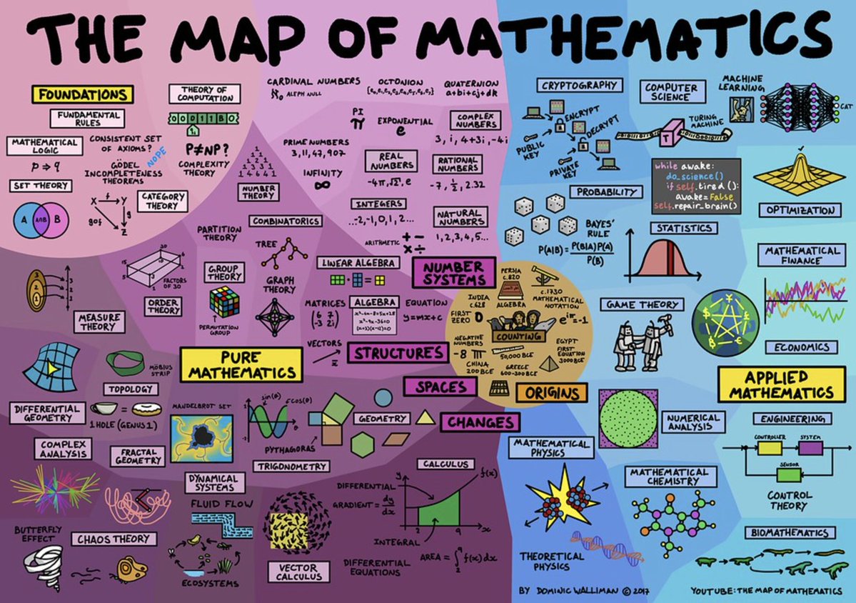
In computer science—a field that many argue is just a branch of mathematics—a handful of mathematical topics are particularly important. These include the Foundations of Mathematics, since it was the so-called “foundational crisis of mathematics” that literally led to the birth of computer science. Let’s begin there.
Foundations
We want to put math on a solid foundation so we know that we are not talking nonsense.
Here’s part of the Wikipedia article on the foundations of mathematics:
Foundations of mathematics are the logical and mathematical frameworks that allow the development of mathematics without generating self-contradictory theories, and to have reliable concepts of theorems, proofs, algorithms, etc. in particular. This may also include the philosophical study of the relation of this framework with reality.
If we can reduce everything down to a few very basic concepts and rules that people can agree upon, then show how to carefully and systematically derive all of mathematics from them, building things up in a way everyone can agree is valid, we can have confidence that mathematics does what it is supposed to do.
Whether you believe philosophically that this is possible or not doesn’t matter for now. What matters is putting in the effort to build a foundation and learning from the effort. Honestly, some fascinating discoveries and useful inventions have come from past work in foundations.
History of Foundations
What we now understand to be the foundations of mathematics today are relatively recent developments, primarily from the late 19th and early 20th centuries. Prior to this time, most of what mathematicians did was just taken for granted. But the the late 1800s and early 1900s saw a rise surprising and paradoxical conclusions from relatively benign claims, and debates about the nature of mathematical truth, leading to what’s now known as the foundational crisis of mathematics.
Several schools of thought emerged to address the foundational crisis. The three main schools were logicism, which aimed to reduce mathematics to logic; formalism, which sought to establish a consistent set of axioms and rules for mathematics; and intuitionism, which emphasized the mental construction of mathematical objects and rejected non-constructive proofs.
Logicism
Math is just logic
Formalism
Math is done by manipulating symbols according to rules
Intuitionism
Math is only what we invent and can construct or demonstrate
Today, this crisis pretty much considered resolved. In the decades of work to complete the resolution, the new field of mathematical logic was born, as were (1) modern versions of Set Theory, Type Theory, and Category Theory, which provide rigorous foundations for mathematics, (2) practical theories such as proof theory, model theory, computability theory, and complexity theory, and (3) the field of computer science itself.
Why Study Foundations?
Good question! Many mathematicians don’t pursue a deep understanding of the foundations of math because they don’t need it in their daily work. But the field turns out to be really useful for computation, theoretical computer science, formal verification of program correctness (used in computer security), and proving complex theorems with the aid of a computer. In other words, it’s important for computer science, particularly in the study of programming languages.
Mathematical foundations underline much of computer science.
And actually, there is some mind-blowing stuff here.
Foundational Theories
There are many theories within mathematics. But there are three kinds of theories that can be viewed as providing a foundation for (all of) math: set theories, type theories, and category theories.
See the Wikipedia page on Foundations of Mathematics and the SEP article on Philosophy of Mathematics for a history of the subject.
Oversimplifying a bit, here’s a bit about these three theories (or technically, theory families):
| Set Theory | Type Theory | Category Theory | |
|---|---|---|---|
| Philosophy and Approach | Math is about classification of objects by arranging them in sets. Set Theory requires logic (generally a classical one) to already exist. | Math is about manipulating objects according to the types they inhabit. Logic emerges from the theory. Usually constructive in nature (though classical type theories do exist). | Math is about structures and the relationships between them, without worrying about internal details. |
| Key Features | Sets are built up from smaller sets, with rules to avoid paradoxes. Generally, everything is a set, which is both a strength and a weakness. | Terms have types. Types can depend on other types as well as on terms. Propositions are types. Proofs are programs. | Categories have objects and morphisms (arrows or relationships). Functors map between categories. Commutative diagrams are used a lot. |
| Concepts | Elements, membership, subsets, power sets, tuples, sequences, partitions, relations, equivalence relations, orders, cardinality. | Types, terms, inductive types, sums ($+$), products ($\times$), dependent types ($\Pi$ and $\Sigma$), propositions as types, proofs as programs, equality types, universes. | Objects, morphisms, functors, natural transformations, limits, colimits, adjunctions, monads, categories, monoids, topoi. |
| Characteristic Notation | $x \in S$ means $x$ is an element of set $S$. | $x : A$ means the term $x$ is of type $A$. | $X \xrightarrow{f} Y$ means $f$ is a morphism from category $X$ to category $Y$. |
| Applications | Used everywhere—most mathematicians are familiar with much of it. | Computer science, formal verification, proof assistants. | Abstract algebra, topology, geometry, mathematical logic. |
| Exemplars | Some set theories are: ZF and ZFC, NBG, NF and NFU, MK, KP, CST. | Some type theories are: Simply-Typed $\lambda$ calculus, MLTT, System F, DTT, CoC, HoTT. | Some category theories are: ETCS, Topos Theory, Abelian, Monoidal. |
Math and LogicMath and logic are related, but not the same thing. Mathematicians do quite a lot of logic. If interested, I have more extensive notes that get into logic in more detail, with coverage of non-bivalent, intuitionistic, paraconsistent, fuzzy, non-monotonic, and a bunch of other types of logic. They get into metalogical notions of soundness and completeness, too.
Mathematical Objects
Mathematics is concerned with objects and the relationships between them, with a focus on the laws the objects obey.
Computer Science is concerned with objects and the relationships between them, with a focus on the behavior of the objects and the processes that manipulate them.
Let’s take an inventory of the kinds of things that humans work with in mathematics that show up often in computer science. We’ll look both at laws and behaviors, since both views are isomorphic. In no particular order, here’s an incomplete sampling of useful mathematical objects:
Booleans Numbers Tuples Sets Relations Functions Sequences Lists Characters Strings Maps Graphs Vectors Matrices Tensors
Let’s visit the basic ideas behind some of these objects.
Booleans
The boolean objects are exclusively $\textsf{true}$ and $\textsf{false}$. They obey several laws, including:
A computational view might be that $\land$ and $\lor$ are operations. But again, the laws and the operations are two sides of the same coin.
Numbers
Numbers are useful. Seriously. We use them to count, measure, order, compare, and so much more.
Some people love numbers. Some numbers have a lot of fascinating properties. Some are interesting philosophically and recreationally. If you like numbers, or even if you think you don’t, browse Robert Munafo’s pages on notable numbers. Then you will like numbers too!
Kinds of Numbers
Numbers are classified by how we use them. Here is a small sampling:
| Type | Concept | What it tells us |
|---|---|---|
| Cardinal Numbers | Quantity | How many discrete items |
| Ordinal Numbers | Sequence | The position of something in an ordering |
| Scalar Numbers | Magnitude | How much (continuous quantity) of something there is |
| Coordinate Numbers | Location | Numbers that represent a position in space |
| Vector Numbers | Direction and Magnitude | Which way and how far |
| Nominal Numbers | Identification | A convenient label |
Here is another way to classify numbers:
| Kind | Symbol | Informal Description |
|---|---|---|
| Natural Numbers | $\mathbb{N}$ | $\{0, 1, 2, 3, \ldots\}$ |
| Integers | $\mathbb{Z}$ | $\{\ldots, -3, -2, -1, 0, 1, 2, 3, \ldots\}$ |
| Rational Numbers | $\mathbb{Q}$ | $\{\frac{a}{b} \mid a, b \in \mathbb{Z} \land b \neq 0\}$ |
| Real Numbers | $\mathbb{R}$ | (See the Wikipedia article) |
| Complex Numbers | $\mathbb{C}$ | Has 2 real components, written ($a+bi$) |
| Quaternions | $\mathbb{H}$ | Has 4 real components, written ($a+bi+cj+dk$) |
| Octonions | $\mathbb{O}$ | 8 real components, with units $e_0 ... e_7$ |
| Sedenions | $\mathbb{S}$ | 16 real components |
There are more! Did you know that algebraic and transcendental numbers were things? This amazing diagram by Keith Enevoldsen shows how they fit in (up to the complex numbers, at least):
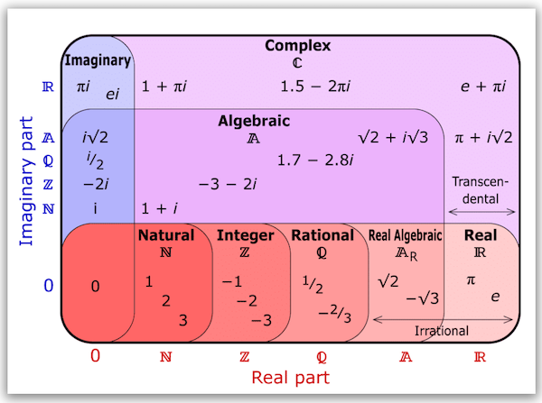
Computable numbers and describable numbers are very useful in computer science theory, but missing from the diagram above. Here is where they land in the real numbers hierarchy:
That’s right! There are real numbers that we can describe but not compute. There are real numbers that exist but that we can’t even describe. This makes computer science (and math) interesting. How we know that we have proper containment at each level of this hierarchy is a little beyond the scope of these notes, but something you should research and internalize at some point.
ΩThe number $\Omega$ in the diagram above is Chaitin’s constant, a number we can describe but not compute. It’s not the same $\Omega$ as the mathematically inconsistent, self-contradictory “absolute infinity” from the Vi Hart video later in these notes.
Things get interesting when you go beyond the reals. What isn’t “real” by the way? Imaginary perhaps? Not a good name, as Jade shows:
Perhaps if they got a better name, the video would have had a different title.
Numeric Operations
Before we get to foundational definitions of numbers, let’s look, informally, at some of the basic operations we can perform with them.
For natural numbers, we define $0$ as the first natural number, and define $\textsf{s}$ as the successor operation:
- Addition: $x^{(1)}y = x + y = \underbrace{\:\textsf{s}\: \ldots \: \textsf{s}\:}_{y}\;x$
- Multiplication: $x^{(2)}y = x \times y = x\cdot y = xy = \underbrace{\:x + x + \ldots + x\:}_{y}$
- Exponentiation: $x^{(3)}y = x^y = x \uparrow y = \underbrace{\:x \times x \times \ldots \times x\:}_{y}$
- Tetration: $x^{(4)}y = {^{y}x} = x \uparrow\uparrow y = \underbrace{\:x \uparrow x \uparrow \ldots \uparrow x\:}_{y}$ (also called hyper4 or power-tower)
- Pentation: $x^{(5)}y = x \uparrow\uparrow\uparrow y = \underbrace{\:x \uparrow\uparrow x \uparrow\uparrow \ldots \uparrow\uparrow x\:}_{y}$
- And on and on....
Addition, multiplication, and exponentiation work for real numbers too. There are also inverses:
- Subtraction: $x - y$ = the $z$ such that $y + z = x$
- Division: $x \div y$ = the $z$ such that $y \times z = x$
- Logarithm: $\log_y(x)$ = the $z$ such that $y^z = x$
- And there are “inverses” of the operators beyond exponentiation as well
Inverse operations need not always exist or be unique for some inputs. For example there is no $z$ such that $0 \times z = 5$, so we say that $5 \div 0$ is not defined.
Got all that? Do you have a good sense of these numbers and operations? You should. Being numerically literate, with a good feel for numbers gives you agency in the world, become less likely to be taken advantage of, and helps you become a better citizen. Watch Vi Hart’s piece which should give you a feel for what having feels about numbers entails:
Also important:
- The floor of a real number $x$, denoted $\lfloor x \rfloor$, is the largest integer less than or equal to $x$.
- The ceiling of a real number $x$, denoted $\lceil x \rceil$, is the smallest integer greater than or equal to $x$.
In computer science, integers, rationals, and reals are often compressed into fixed size registers, yielding classes of bounded numbers. You can study these in more depth in the notes on Numbers and Numeric Encoding.
Big Numbers
Robert Munafo has another catalog of numbers, his Large Numbers pages, which you absolutely don’t want to miss. It includes not only large numbers, but the transfinite ordinals.
Seriously, don’t miss it!
Have ten hours to spare? This will take you through large finite numbers only, but in doing so, will give you a sense that thinking that infinity is not a big deal isn’t really accurate. Though easy to describe, it’s so far beyond direct experience. You just can’t.
If you want to become immersed and well-versed in this stuff, start at the Googology Wiki. Have fun!
One small nitThis video seems to suggest that infinity is a number, which isn’t really accurate. Infinity is not a number, but there are numbers that represent infinities in various mathematical contexts.
Infinities
There are not only so many kinds of numbers but there are even many kinds of transfinite numbers. Perhaps you encountered a few of these already in Robert Munafo’s Large Numbers pages. Whether you have or have not, Vsauce gives a careful explanation of cardinals (“how many”) and ordinals (“position of”) that really helps!
Vsauce does not go far enough. Vi Hart takes us much, much further:
So many types of numbers in this video: cardinals in Set Theory, surreals in Game Theory, supernaturals in Field Theory, ordinal spaces in Topology, Hilbert spaces in Analysis and Quantum Physics, and more.
Many of the infinities are best understood in the context of Set Theory. So we’ll defer a proper treatment of cardinals and ordinals to our upcoming notes on Set Theory.
Infinity and EthicsNick Bostrom has an essay discussing the ethical implications of dealing with infinite populations and resources. Infinity is a wild concept. Give the paper a read.
Pairs
A pair, also called an ordered pair, is an object $(a, b)$ where $a$ is the first element and $b$ is the second element. The order of the elements matters, meaning that the pair $(a, b)$ is only the same as the pair $(b, a)$ when $a = b$.
Pairs are a fundamental building block for more complex structures.
Tuples
A tuple is an object such as $(21,F)$, $(a,a,b,a,b,a,b,b)$, or $(do, re, mi, fa, so, la, ti, do)$. The elements of a tuple are ordered. Given a tuple $t$, you access the $i$th element with the notation $\:t\!\downarrow\!i$.
Tuples are just pairs. For example, The $3$-tuple $(a, b, c)$ is the pair $(a, (b, c))$, and a the $4$-tuple $(a, b, c, d)$ is the pair $(a, (b, (c, d)))$, and so on. Tuple notation is just sugar for the true, underlying pair notation.
In general, $(a_1, \ldots, a_n)$ sugars $(a_1, (a_2, (\ldots, (a_{n-1}, a_n)\ldots)))$ and is called an $n$-tuple. Its length is $n$. Because tuples are pairs, every tuple has a length of at least $2$.
That said, we can get a little informal, and speak of $1$-tuples and $0$-tuples, too. The convention is $a = (a)$ for a $1$-tuple and the $0$-tuple is simply $()$.
Tuples can be concatenated. If $t_1$ is an $m$-tuple and $t_2$ is an $n$-tuple then $t_1 • t_2$ is an $(m+n)$-tuple:
$$(a_1, \ldots, a_m) • (b_1, \ldots, b_n) = (a_1, \ldots, a_m, b_1, \ldots, b_n)$$We will allow the concatenation operator to work with $0$-tuples and $1$-tuples as well, so $(a,b) • c = (a,b,c)$, $a • b = (a,b)$, and $a • () = a$.
Sets
A set, in practice, is an unordered collection of unique elements. We denote sets by (1) enumerating their elements or (2) using a filtering notation to select certain elements from an existing set. (This restriction is important because only certain collections are allowed to be sets—more on this when we study set theory later.) You can use prose as long as the precise meaning can be recovered exactly and uniquely.
Crisp and Fuzzy SetsWhat does it mean to be a member? It can vary.
- For crisp sets, you’re either in or you’re out. No in-between. This is the most common kind of set.
- For fuzzy sets, membership can be partial. For example, you might be 0.8 in the set of tall people.
These notes will only cover crisp sets.
Set Notation
There is a lot of notation surrounding sets:
AMBIGUOUS NOTATION ALERT: $A^n$The notation $A^n$ is horribly overloaded! When $A$ is a plain old set, the notation indicates tuple construction, as shown above. When $A$ is a relation or function (terms we’ll define later), the notation indicates repeated composition. When $A$ is an alphabet (also something we’ll define later), the notation indicates the set of strings with a given length. When $A$ is a language (you guessed it, something we’ll define later), the notation indicates sets of strings made by concatenating strings from $A$ a given number of times.
In each of these cases, the value of $A^n$ is completely different!
Context is crucial to understanding the meaning. Ambiguity is very common in math. Math is supposed to be convenient for humans, not rigid, so do not be surprised if something is ambiguous and confusing.
A Few Laws of Sets
Assuming you already know first-order classical logic, you can use the definitions above to prove some interesting laws that sets obey. The following are theorems of all the major set theories. They hold for any arbitary $A$, $B$, $C$, and $D$.
Disjointness and Partitions
A notion that comes up often when working with sets is that of separating out the elements of a set into non-overlapping groups. Two technical terms are useful here.
$A$ and $B$ are disjoint iff $A \cap B = \varnothing$
$\Pi = \{P_1, P_2, \ldots, P_n\} \subseteq \mathcal{P}(A)$ is a partition of $A$ iff:
- $\varnothing \notin \Pi$
- $\forall x\:i\:j. (x \in P_i \land i \neq j) \supset x \notin P_j$
- $\bigcup \Pi = A$
Relations
When we say “Five is less than eight” we are expressing a relation between two numbers. You can probably think of many more, For numbers, we have $\leq$, $\gt$, and $\geq$. For sets, there is $\subseteq$. For people, the relation “likes” comes to mind.
When $a$ is related to $b$ by a relation $R$, we write $aRb$.
Kinds of Relations
Relations appear everywhere, so people have found it useful to identify some common kinds of relations:
- $R$ is reflexive iff $\forall a. aRa$
- $R$ is irreflexive (a.k.a anti-reflexive) iff $\forall a. \neg aRa$
- $R$ is symmetric iff $\forall a\:b. aRb \supset bRa$
- $R$ is asymmetric iff $\forall a\:b. aRb \supset \neg bRa$
- $R$ is antisymmetric iff $\forall a\:b. aRb \land bRa \supset a=b$
- $R$ is transitive iff $\forall a\:b\:c. aRb \land bRc \supset aRc$
- $R$ is total iff $\forall a\:b. aRb \vee bRa$
And some more:
- $R$ is an equivalence relation iff it is reflexive, symmetric, and transitive
- $R$ is a partial order iff it is reflexive, antisymmetric, and transitive
- $R$ is a total order iff it is antisymmetric, transitive, and total
The relation $=$ should be defined for every kind of object.
Woah. What is this $=$ relation?Even though we had been using $=$ all along, it’s not something that already exists for free: the equality relation has to be defined, and it is generally defined differently for each type of mathematical object. Definitions like the following are widely accepted:
- For booleans, $x=y$ iff $x$ and $y$ are both true or both false
- For natural numbers, $x=y$ iff $x$ and $y$ are the same number
- For sets, $X=Y$ iff $X$ and $Y$ have exactly the same elements
- ...and so on.
There is an expectation that an equality be reflexive, symmetric, and transitive. If you have programmed in JavaScript before, you may now see why calling the infamous
==operator “equals” is so horrific and a violation of one of the most sacred principles of philosophy, mathematics, and human well-being. It is unabashedly nontransitive, and therefore it does not even pretend to be an equivalence relation. Call it “similar to” instead.
Composition of Relations
Relations can be composed: If $aRb$ and $bSc$, then $a$ is related to $c$ by the composed relation $S \circ R$. The $\circ$ symbol is read ”after”, since we look at $S$ after $R$. It can be proven that composition is associative, which allows us to write things like $R \circ R \circ R \circ R$ without parentheses. An in yet another overloading of notation, you’ll find $R^n$ used for the $n$-fold composition of $R$ with itself, so $R^1 = R$, $R^2 = R \circ R$, $R^3 = R \circ R \circ R$, and so on. There’s also $R^*$, which means related to in any nonnegative number of steps, including $0$.
Wait...nonnegative? What is $R^0$? What is $R^{-1}$? Relations are frequently used in computation theory to describe state changes in nondeterministic systems. The relation is sometimes called a transition relation and denoted by $\longmapsto$ so you’ll see something like $\psi_1 \longmapsto \psi_2$ meaning the computation system can move from state $\psi_1$ to state $\psi_2$. So $R^0$ is taking no steps, and $R^{-1}$ is taking one step backwards.
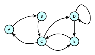
and
$R^{-1}$ has a name: the inverse relation.
Functions
A function maps an input to an output, such that given any input (called the argument), you get the same output every time you apply the function.
To apply or invoke the function $f$ on argument $a$, we write $f\,a$ or $f(a)$. To represent a function explicitly, we write:
where $x$ is the parameter of the function and $e$ is the expression that computes the output based on $x$.
Pay attention: $f$ is a function but $f(x)$ is the result of applying the function. So $f(x)$ is emphatically not the function itself, but rather the output of applying the function.
AMBIGUOUS LANGUAGE ALERT: $f(x)$If $f$ is a function, do not say “the function $f(x)$” unless the function $f$, when applied to $x$, actually yields a function. Also do not say things like “the function $n^2$” because $n^2$ is a number. The function you probably have in mind is $\lambda n. n^2$. That doesn’t stop people from abusing the notation, though.
Mathematics is often about communicating ideas, not about absolute precision. Confusing people is part of the fun of math, it seems. Context matters. When something is ambiguous, ask about it.
Let and Where
Here are some powerful readability aids:
$\begin{array}{lll} \textsf{let}\;x = e\;\textsf{in}\;e' & \text{sugars} & (\lambda x.\,e')\;e \\ e'\;\mathsf{where}\;x = e & \text{sugars} & (\lambda x.\,e')\;e \end{array}$
Examples of $\textsf{let}$:
- For example: $\;\mathsf{let}\;x=3\;\mathsf{in}\;x+5$ evaluates to $8$
- Because: $\;\mathsf{let}\;x=3\;\mathsf{in}\;x+5$ is the same as $(\lambda x . x+5)(3)$
- In general: $\;\mathsf{let}\;x=e\;\mathsf{in}\;e'$ is the same as $(\lambda x . e')(e)$
Examples of $\textsf{where}$:
- For example: $\;x+5\;\mathsf{where}\;x=3$ evaluates to $8$
- Because: $\;x+5\;\mathsf{where}\;x=3$ is the same as $(\lambda x . x+5)(3)$
- In general: $\;e'\;\mathsf{where}\;x=e$ is the same as $(\lambda x . e')(e)$
Untyped and Typed Functions
A function that is allowed to map any object to any object is called an untyped function. An example is $\lambda x. x\,x$, which is interesting because applying to itself doesn’t evaluate to anything because it produces the never-ending computation:
$\begin{array}{lcl} (\lambda x. x\,x)\,(\lambda x. x\,x) & = & (\lambda x. x\,x)\,(\lambda x. x\,x) \\ & = & (\lambda x. x\,x)\,(\lambda x. x\,x) \\ & = & (\lambda x. x\,x)\,(\lambda x. x\,x) \\ & = & \ldots \end{array}$
Another is $\lambda x. \neg(x\,x)$, whose computation when applied to itself yields the somewhat unpleasant:
$\begin{array}{lcl} (\lambda x. \neg(x\,x))\,(\lambda x. \neg(x\,x)) & = & \neg((\lambda x. \neg(x\,x))\,(\lambda x. \neg(x\,x))) \end{array}$
To see why it is unpleasant, let $R = \lambda x. \neg(x\,x)$ and note that $R\,R = \neg(R\,R)$. Ugh—a mathematical object equal to its own negation. Untyped functions are fine for describing computations, but they are not suitable for building a consistent foundation for mathematics. They are fun when considering paraconistency, though.
A typed function declares beforehand a restriction of its input to a particular domain and a restriction of its output to a specific codomain. The domain and codomains can be either types (in Type Theory) or sets (in Set Theory). If the domain is $A$ and the codomain is $B$, the function is an inhabitant or member of $A \rightarrow B$. Usually the output type or set is inferrable, so we annotate only the parameter, as in $\lambda x_t. e$ or $\lambda x:\!T. e$ in Type Theory and $\lambda x\in S. e$ in Set Theory.
Some examples:
It’s pretty cool that the logical operators can be defined as functions. This turns out to by why Type Theory is used as a foundation for mathematics, and unlike Set Theory, does not require logic to already exist. We can even go further: sets can be modeled as functions that return booleans, and relations can be modeled as functions returning sets. (We will explore why this is so when we discuss Type Theory in detail.)
Here’s a shorthand notation you might like. If your function does a case analysis on its argument immediately, you can elide the argument. Here’s the boolean negation function as an example:
$ \lambda(\mathsf{true} \to \mathsf{false} \mid \mathsf{false} \to \mathsf{true}) $
$\lambda(\mathsf{true} \to \lambda y_\textsf{Bool}. \mathsf{true} \mid \mathsf{false} \to \lambda y_\textsf{Bool}. y)$
Naming Functions
We often give (readable) names to functions, for example:
There’s a shortcut definition (called definition by cases) that lets you elide the $\lambda$:
The Conditional Function
This function is remarkably useful:
$ \textsf{cond} =_{\small{\textrm{def}}} \lambda b_{\textsf{Bool}}. \lambda x_t. \lambda y_t. [\,b \ \Vert \ \mathsf{true} \to x \mid \mathsf{false} \to y\,] $
If you prefer the shorthand notation, you can write it as:
$ \textsf{cond} =_{\small{\textrm{def}}} \lambda(\mathsf{true} \to \lambda x_t. \lambda y_t. x \mid \mathsf{false} \to \lambda x_t. \lambda y_t. y) $
There is a more common sugared notation for this function:
$\begin{array}{lcl} \textsf{if}\;b\;\textsf{then}\;x\;\textsf{else}\;y & \text{ sugars } & \textsf{cond}\;b\;x\;y \end{array}$
Here it is in action:
$\begin{array}{lcl} \textsf{abs}\;x_{\textsf{Int}} =_{\small{\textrm{def}}} \textsf{if}\;x \ge 0\;\textsf{then}\;x\;\textsf{else}\;(-x)\\ \textsf{sign}\;x_{\textsf{Int}} =_{\small{\textrm{def}}}\; \textsf{if}\;x > 0\;\textsf{then}\;1\;\textsf{else}\;(\textsf{if}\;x \lt 0\;\textsf{then}\;{-1}\;\textsf{else}\;0) \end{array}$
Polymorphism and Overloading
The $\textsf{cond}$ function we defined above is an example of a polymorphic function. It can operate on any type $t$, not just a specific type like $\textsf{Nat}$ or $\textsf{Bool}$. This is powerful. Many programming languages make use of this idea.
The word comes from the Greek words poly meaning many and morph meaning form.
You can also think of $\textsf{cond}$ as being a template for an infinite number of functions, one for each type. This kind of polymorphism is truly universal, as it applies to every $t$. In fact, we sometimes use the universal quantifier in expressing the type of $\textsf{cond}$ as $\:\forall t.\;\textsf{Bool} \rightarrow t \rightarrow t \rightarrow t$.
Now some symbols and operators, like $+$, $\times$, and so on will be used across multiple arithmetic types, and perhaps on nonarithmetic types too. Not all types, just some types. Here we’re using a single function name or operator across multiple types to carry out what are often fundamentally distinct functions. It’s certainly not the universal polymorphism of $\textsf{cond}$. Instead, it is just a convenient way to say “these operations are pretty similar across a handful of types so we will overload the name.”
Modification
Sometimes we have a function $f$ and want to make a function that behaves like $f$ except for some specific input value. We have a notation for that:
$f[a \mapsto b] = \lambda x. \mathsf{if}\;x=a\;\mathsf{then}\;b\;\mathsf{else}\;f(x)$
Composition of Functions
The operator $\circ$ is pronounced “after,” i.e., $f \circ g$ is the function that applies $f$ after applying $g$:
- $(f \circ g)(x) = f(g(x))$
Function iteration is the repeated application of a function to its own output, or, equivalently, repeated self-composition:
- $f^0(x) = x$
- $f^1(x) = f(x)$
- $f^2(x) = f(f(x))$
- $f^3(x) = f(f(f(x)))$
- ...
- $f^{n+1}(x) = f(f^n(x))$
Fun fact: If $f$ is a function, then $f^n$ is also a function if $n\ge 0$. But if $n \lt 0$, $f^n$ won’t be the same kind of function, since in “going the other way” a value may map to zero, one, or many values.
AMBIGUOUS NOTATION ALERT: $sin^2\theta$Many mathematicians purposefully blur the distinction between $\sin^2\theta$ and $(\sin \theta)^2$, leaving you, the poor reader, to figure out what they mean by context. It can be very annoying.
It appears that for trigonometric functions, people tend to use the iterative form for the power form, but for other functions the iterative form usually means iteration. Maybe?
Don’t worry too much. It’s all a consequence of the fact that everyone is allowed to invent their own notation. Just remember, all things are contextual.
Matching
Given a typed function $f$ with domain $A$ and codomain $B$, we’re often interested in how the inhabitants or members of $A$ and $B$ match up. There are three really interesting cases:
- $f$ is an injection (1–1) iff every $a$ in the domain is mapped to an exclusive $b$ in the codomain
- $f$ is a surjection (onto) iff every $b$ in the codomain is the image of some $a$ in the domain
- $f$ is a bijection iff $f$ is an injection and a surjection
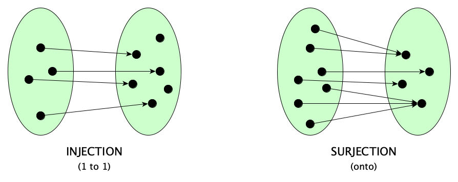
Why do we care? In computer science, at least:
- Injections (unique outputs) are related to preventing data collisions in hashing functions and database keys, and for processes needing to recover the original inputs if things go awry.
- Surjections (full output coverage) are used in proving that an equation or system has a valid solution for every possible target value.
- Bijections (perfect pairings) serve as the gold standard to prove two sets have the exact same size, and express structure-preserving relationships and other forms of equivalences.
Partial Functions
Here’s something that might happen. You declare a typed function with domain $A$ and codomain $B$, but not every element in $A$ has an image in $B$. In this case, the function is called a partial function. The type or set of partial functions from $A$ to $B$ is often written as $A \rightharpoonup B$. When partial functions are under consideration, the term total function is used to refer to functions that are defined for every element in the domain.
Partial functions are useful in computer science because they allow us to model programs that might not terminate, crash, or produce an error rather than a result of the expected type. However, many modern programming languages are adopting the “errors-as-values” approach: for functions that may fail, we use total functions whose codomain is a sum or union type combining expected return values and error values. For functions that never terminate, partial functions remain useful.
Function Equality
What about function equality? Given two functions $\lambda x. e_1$ and $\lambda y. e_2$, which we’ll call $f$ and $g$, we can call them equal (1) if and only if the two expressions are formulated exactly the same way, or (2) if and only if for all inputs $x$, $f(x) = g(x)$. The first notion is called structural equality, and the second is called extensional equality.
We’ll always assume $=$ means extensional equality, unless otherwise specified.
Sequences
A sequence $\langle a_0, a_1, a_2, \dots, a_{n-1} \rangle$ is an ordering of $n$ elements indexed by the natural numbers $0, 1, 2, \dots, n-1$, where $n$ is the length of the sequence. Operations on sequences including lookup by position and appending:
Both the set-theoretic and type-theoretic encodings of sequences are fascinating. They will be covered later in the course.
Lists
A list is defined inductively like this:
- The empty list $[\,]$ is a list.
- If $x$ is an element and $y$ is a list, then $(x :: y)$ is a list.
This means a list is an ordered collection of elements. This shows in the conventional notation: We write ${[x]}$ for $(x\,\textbf{::}\,[\,])$, ${[x,y,z]}$ for $(x\,\textbf{::}\,(y\,\textbf{::}\,(z\,\textbf{::}\,[\,])))$, and so on.
Lists are particularly useful in mathematics and computer science, and appear in nearly every mainstream programming language. Several dozen useful lists operations are known, among them:
head: Returns the first element of the list if the list is non-empty.tail: Returns the list without the first element if the list is non-empty.++: Concatenates two lists together, end to end.length: Returns the number of elements in the list.map: Applies a function to each element of the list.filter: Returns a list of elements that satisfy a predicate.
Lookup by position and finding the index of an element can also be defined, but such operations are foreign to lists. Lists are not meant to work that way.
Sequences vs. ListsSequences by nature are designed to be indexed by position and are called random access structures. Lists, on the other hand, are inductive, built from the empty list and the prefixing operation
::. List elements are accessed viaheadandtailoperations, rather than by position.
Characters
A character is a primitive unit of textual information. In practice, we create sets of characters called alphabets.
The most common alphabet in the world today is Unicode. Characters in Unicode have both a code point (a unique natural number identifying the character) and a name, such as U+0041 LATIN CAPITAL LETTER A.
The science of characters is quite vast. You can learn by browsing the resources available through unicode.org, or, for a computer science approach, see the course notes on Characters and Character Encoding.
Strings
A string is a list of characters. Sets of strings are called languages. We cover strings and languages in much more detail in our notes on Language Theory, where we will encounter a great many operations.
Maps
A map, or dictionary, is a lookup table, commonly written like a set whose elements are labeled with the keys of the map, which must be distinct (or if not distinct, with later bindings overriding earlier ones):
$ \{ \texttt{a}\!: 1, \texttt{b}\!: 2, \texttt{c}\!: 3 \}$
Maps are constructed from the empty map by adding key-value pairs. The empty map is generally written as $\{\}$. add or update a key-value pair in a map, we use the notation $m[\textit{key} \mapsto \textit{value}]$. So the map expression we saw above is actually sugar for:
$ \{\}[\texttt{a} \mapsto 1][\texttt{b} \mapsto 2][\texttt{c} \mapsto 3] $
The characteristic operation is lookup by key. For the map $m = \{ \texttt{a}\!: 1, \texttt{b}\!: 2, \texttt{c}\!: 3 \}$:
Graphs
Structurally, a graph consist of vertices and edges connecting pairs of vertices. Here’s an example:
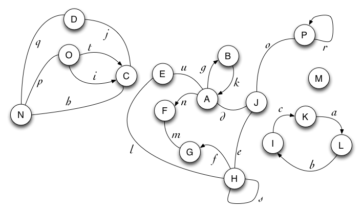
Behaviorally, a graph comes with associated operations such as finding paths, computing connectivity, traversal and much more. Rather than looking at definitions, here’s terminology introduced by example:
- The order of the graph is 16, because it has 16 vertices, $A$...$P$.
- The size of the graph is 21, because it has 21 edges, $a$...$u$.
- $h$ is an undirected edge, whose endpoints are $N$ and $C$.
- $f$ is a directed edge, whose tail is $H$ and whose head is $G$.
- $t$ and $i$ are parallel edges; $g$ and $k$ are antiparallel edges.
- $r$ and $s$ are loops; all the other edges are links.
- $M$ is an isolated node.
- $J$ is an articulation point.
- $o$ is a bridge.
- $C$ and $D$ are adjacent.
- $C$ and $j$ are incident.
- $G$ has degree 2; $H$ has degree 5.
- $A$ has degree $5$, indegree 1, and outdegree 2.
- $\langle PrPoJdAgBkAuEuAnF\rangle$ is a walk of length 8, start $P$, and end $F$.
- $\langle PrPoJdA\rangle$ is an open walk.
- $\langle PrPoJeHsHeJoP\rangle$ is a closed walk.
- $\langle AdJeHfG\rangle$ is a path (open walk with no repeated vertices).
- $\langle OtChNpO\rangle$ is a cycle (closed walk of length>0 with no repeated vertices other than the first/last, and no repeated edges).
- $\langle OtChNpOiCjD\rangle$ is a trail (open walk with no repeated edges)
- $\langle AgBkAuElHeJdA\rangle$ is a tour (closed walk with no repeated edges)
- The graph is not connected; it has 4 blocks.
There are a few terms that apply only to connected graphs. Consider the block in the graph above containing vertices $\{D, C, O, N\}$ and edges $\{q, p, h, i, t, j\}$:
- $\langle OiCjDqN\rangle$ is a Hamilton Path (Hamiltonian: all the vertices).
- $\langle DqNpOtCjD\rangle$ is a Hamilton Cycle.
- $\langle OtChNpOiCjDqN\rangle$ is an Euler Trail (Eulerian: all the edges).
- The block has no Euler Tour.
The next three objects form a natural progression. A scalar is just a number. A vector is a 1-dimensional array of numbers. A matrix is a 2-dimensional array. A tensor generalizes all of them to any number of dimensions. Structurally, each is just a (nested) tuple of numbers; what makes each one interesting is the operations and laws that come along for the ride.
Vectors
Structurally, a vector is a tuple that contains numbers, that adhere to certain operations, among them are (where $\vec u, \vec v, \vec w$ are vectors and $c, d$ are scalars):
From these definitions, you’ll note various laws:
Zero-based IndexingAs we did with tuples and sequences, the first index of a vector element is $0$, not $1$. $0$-based indexing is much more common in computation, as it is for matrices and tensors. The $0$-based indexing is used in computer graphics, game engines, machine learning, data science, numerical analysis, and scientific computing.
Matrices
Structurally, a matrix is a two-dimensional array of numbers. Behaviorally, a matrix comes with associated operations obeying the laws of matrix algebra.
A matrix with $m$ rows and $n$ columns is called an $m \times n$ matrix. As with vectors, addition of matrices and scalar multiplication is component-wise. Multiplication is a little different. To compute $A$ times $B$, you must have that $A$ is an $m\times k$ matrix and $B$ must be a $k \times n$ matrix. The result is an $m \times n$ matrix $C = AB$, where each element $c_{ij}$ is computed as the dot product of the (zero-indexed) $i$th row of $A$ and the (zero-indexed) $j$th column of $B$.
Matrix multiplication is not commutative. In general, $AB \neq BA$.
Here are a few representative laws, where $A$, $B$, $C$ are matrices and $I$ is the identity matrix:
Tensors
Structurally, a tensor is a multi-dimensional array of numbers, generalizing scalars (rank 0), vectors (rank 1), and matrices (rank 2) to any rank $n$. Behaviorally, addition and scalar multiplication generalize the same way they do for vectors and matrices, component-wise across however many indices the tensor has:
Wait, what exactly is a tensor?In mathematics, not just any array of numbers is a tensor. A genuine tensor is defined by how its components transform under a change of coordinates, not merely by its shape. In computer science, however, the term is used loosely for any $n$-dimensional array (as in a “tensor” in PyTorch or TensorFlow).
Proofs and Programs
Much of mathematics is aided by the use of computers. Computers speed up time, allowing us to think previously unthinkable thoughts. Computers make science and mathematics qualitatively different. Computers augment and amplify human thought. In math, complex proofs can be found or checked by automated proof assistants.
Generally, these proof assistants are based on Type Theory, not Set Theory, for various reasons (many taken from these slides by Sergey Goncharov):
- In Type Theory, functions are primitive. They are not just special kinds of sets of pairs. Functions compute things, and thus feel dynamic. Why look at them like static relations?
- Set Theory purports to be simpler, in that it has fewer basic notions, as in everything is a set. But this really isn’t the case, as the axioms of Set Theory are really complex and few people know them all. The axioms are arguably arbitrary and don’t help much in finding proofs. Set Theory is just too theoretical.
- Set Theory’s “everything is a set” approach is actually too simple. We want to distinguish tuples and functions and relations and numbers. Mathematicians naturally think in terms of different types of objects. Why treat them all as sets? This leads to silliness like $2 \in 3$ and $\pi \cap \mathbb{R}$.
- In Set Theory, logic and objects come first, then we use sets to group the objects. In Type Theory, types come first, then we construct objects to inhabit the types, and logic emerges. Thus Type Theory does not decouple logic from the objects it defines the way Set Theory does.
- Most type theories are constructive! There’s no excluded middle, for one thing. To prove existentials, you have to supply a witness. To prove disjunctions, you have to show one of the disjuncts. Computation feels constructive. In contrast, most set theories are classical.
- Set Theory’s underlying logic has debatable principles such as the Excluded Middle, the Axiom of Choice, and Impredicativity, which get in the way of automation.
Remember how we started with the observation that Logic is a prerequisite for Set Theory, but Logic emerges from Type Theory? Perhaps this means Type Theory is more fundamental? Maybe. But it does indicate something: there must be a deep connection between Logic and Type Theory.
We won’t cover it all right now, but will leave you with something to think about. Here is the type inference rule that tells us the type of the output of a function application:
That looks like Modus Ponens in logic. Is that a coincidence or an interesting correspondence?
And the inference rule for inferring the type of a pair is:
Can’t you just feel logical conjunction here?
This is just a small part of the Curry-Howard correspondence, which we’ll see when we cover Type Theory in depth.
Additional Topics
Our focus on this page has been on introducing the notation and fundamental mathematical objects that play a large role in computation. But there’s much more to math that is useful in computer science. You might want to check out:
- Counting principles (pigeonhole, addition, multiplication)
- Permutations
- Combinations
- Recurrence Relations
- Algebraic Structures
- Linear Algebra
- Geometry
- Topology
- Analysis
- Probability, for which you really need to see the amazing Seeing Theory: A Visual Introduction to Probability and Statistics
- Optimization
- Graph Theory
- Number Theory
Does Math Describe the World?
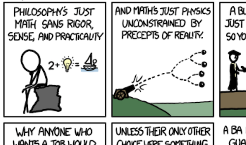
Did you watch the Vsauce video above? Kind of cool how Michael says we can do math that isn’t science and just invent things that we declare to be true, like transfinite infinities, and yeah, as long as we don’t have contradictions, let’s go. The first two frames of the famous XKCD Every Major’s Terrible has fun with this idea:
Sometimes our inventions do give us good models. Cohl Furey explains it in two minutes:
Intrigued? Watch her entire Division Algebras And the Standard Model playlist. Or checkout this article on her work.
Recall Practice
Here are some questions useful for your spaced repetition learning. Many of the answers are not found on this page. Some will have popped up in lecture. Others will require you to do your own research.
- What are some things that are reasoned about within mathematics? Quantity, structure, change, chance, causality, and space.
- Mathematic reasoning involves finding abstract ________________ and constructing ________________ of real and imaginary phenomena. patterns, models.
- Was math invented or discovered? Probably both.
- What are some of the main branches within mathematics? Foundations, algebra, analysis, discrete, geometry, number theory, topology, applied mathematics, and computational mathematics.
- When was the foundational crisis of mathematics and what was it? Early 20th century. Mathematicians discovered contradictions in some of the naïve foundational theories and were not completely sure of the soundness and completeness of many others.
- What are three theories that claim to be able to formalize “all of mathematics”? Set Theory;
Type Theory;
Category Theory. - What three schools arose to address the foundational crisis? Logicism, Formalism, Intuitionism.
- What are the characteristic notations of set, type, and category theory? $x \in A$
$x : A$
$X \xrightarrow{f} Y$ - What is perhaps the main difference between Set Theory and Type Theory? In set theory, everything is a set. In Type Theory, types come first, and objects are constructed to inhabit the types.
- What are some of the foundational mathematical objects? Booleans, numbers, tuples, characters, strings, sequences, relations, functions, sets, vectors, matrices, tensors, maps, graphs.
- What are the boolean values? true, false
- What does the notation $x \supset y$ mean, where $x$ and $y$ are boolean values? It is the same as $\neg x \lor y$, in other words either $x$ is false or $y$ is true.
- Who is the guy that made that freaking amazing set of web pages on big numbers? Robert P. Munafo
- What is cardinal number? A number that tells you how many of something there is.
- How are ordinal numbers different from cardinal numbers? Ordinal numbers describe the position of an element in a sequence, while cardinal numbers describe the size of a set.
- How do cardinal and scalar numbers differ? Cardinal numbers indicate discrete quantity, while scalar numbers indicate magnitude.
- What kind of number is this: $3 + 8i - 5j + k$? A quaternion.
- What kind of a number is $2 - 5e_0 * 8e_6$? An octonion.
- What do we call $\uparrow$, $\uparrow\uparrow$, and $\uparrow\uparrow\uparrow$? Exponentiation, tetration, pentation.
- How do you conventionally write $5 \uparrow\uparrow 3$? $5^{5^5}$
- Perform “one-step” in the simplification of $8 \uparrow\uparrow\uparrow 5$. That is, write the expression in terms of the $\uparrow\uparrow$ operator alone. $8 \uparrow\uparrow\uparrow 5 = 8 \uparrow\uparrow (8 \uparrow\uparrow (8 \uparrow\uparrow (8 \uparrow\uparrow 8)))$
- What are the ”inverses” of addition, multiplication, and exponentiation? Subtraction, division, logarithm.
- What is $\log_2 1024$ and why? $10$, because $2^{10} = 1024$
- What is $\log_{2} 0.125$ and why? $-3$, because $2^{-3} = \frac{1}{2^3} = \frac{1}{8} = 0.125$
- How do we write “three-fourths of the way to 81 in a times-ish counting way?” $81^{\frac{3}{4}}$
- What is a trotillion? (You’ll need to look this up or find it in the Big Numbers video) $10^{(3 \times 10^{(3 \times 10^{900})} + 3)}$
- What does a tuple look like? $(a, b, c)$
- What is $(10, 20, 30)\downarrow 1$? $20$
- What is $(2, 8, 3) \bullet (5, 1)$? $(2, 8, 3, 5, 1)$
- What does the expression $A \subseteq B$ sugar? It is syntactic sugar for $\forall x (x \in A \rightarrow x \in B)$.
- How do sets differ from tuples? Sets are unordered and do not contain duplicates.
- What is the difference between a crisp set and a fuzzy set? A crisp set is a set where an element is either in the set or not. A fuzzy set is a set where an element can be partially in the set.
- How do we denote that $x$ is a member of the set $A$? $x \in A$
- Why isn’t $\{ x \mid x \not\in x \}$ considered a set? Considering it a set ruins everything because if it were a set, assuming it was a member of itself would imply it was not and assuming it was not a member of itself would imply that it was.
- How is set subtraction $A \setminus B$ defined? $\{x \in A \mid x \notin B\}$
- What is the difference between $A-B$ and $A \setminus B$? Nothing, they are the same.
- What is the difference between $A \setminus B$ and $A \vartriangle B$? The first is the set of all elements in $A$ but not in $B$. The second, the symmetric difference, is the set of elements that are in exactly one of $A$ or $B$.
- What is $\varnothing \times \varnothing$? $\varnothing$
- What is $\mathcal{P}(\{a,b,c\})$? $\{\varnothing, \{a\}, \{b\}, \{c\}, \{a,b\}, \{a,c\}, \{b,c\}, \{a,b,c\} \}$
- What is $\{1,2\}^*$ (assuming this set is not an alphabet or language)? $\{(), (1), (2), (1,1), (1,2), (2,1), (2,2), (1,1,1), (1,1,2), (1,2,1), (1,2,2), (2,1,1), \ldots \}$
- What is $\{1, 2\}^0$? $\{ () \}$
- What are the distinct partitions of $\{ a, b \}$?
- $\{ \{a\}, \{b\} \}$
- $\{ \{a,b\} \}$
- What are the distinct partitions of $\{ a, b, c \}$?
- $\{ \{a\}, \{b\}, \{c\} \}$
- $\{ \{a,b\}, \{c\} \}$
- $\{ \{a,c\}, \{b\} \}$
- $\{ \{b,c\}, \{a\} \}$
- $\{ \{a,b,c\} \}$
- Are the set of all even integers and the set of all prime numbers disjoint? No, they share the number $2$.
- What is required for a relation to be a total order? Antisymmetry, transitivity, and totality.
- What does it mean for a relation $R$ to be reflexive? $\forall a.\, aRa$
- Give an example of a relation over $\{a, b, c\}$ that is neither reflexive nor irreflexive. $\{(a, a), (b, c)\}$ is not reflexive because it does not contain $(b, b)$, and it is not irreflexive because it does contain $(a, a)$.
- What is the difference between “asymmetric” and “antisymmetric”? An asymmetric relation can never have a member of the form $(x,x)$, but an antisymmetric relation can.
- What are the three properties required for $R$ to be a partial order? Reflexive, antisymmetric, and transitive.
- What are the three properties required for $R$ to be an equivalence relation? Reflexive, symmetric, and transitive.
- If $aRb$ and $bSc$, what relation connects $a$ to $c$, and how do we read the $\circ$ symbol? $S \circ R$; the symbol is read “after” (apply $R$, then $S$).
- What does $R^*$ mean? Related by $R$ in any number of steps, including zero.
- What symbol is conventionally used for a transition relation, and what does $\psi_1 \longmapsto \psi_2$ mean? $\longmapsto$; it means the computation system can move from state $\psi_1$ to state $\psi_2$ in one step.
- How do we denote the type of a function from $A$ to $B$? $A \rightarrow B$
- How do we denote the set of all functions from $A$ to $B$? $A \rightarrow B$
- How do you write let $x = 8$ in $2^x - 1$ without the “let”? $(\lambda x. 2^x - 1)(8)$
- How do you write $(\lambda x. x + 3)(5)$ in where-notation? $x + 3\;\textsf{where}\;x = 5$
- Suppose $f = \lambda x. x^2$ and $g = \lambda x. x + 3$. What are $f \circ g$ and $g \circ f$? $f \circ g = \lambda x. (x + 3)^2$
$g \circ f = \lambda x. x^2+3$ - Suppose $f = \lambda x. 5x + 2$ and $g = f[1 \mapsto 2]$. What are $g(8)$ and $g(1)$? $g(8) = 42$
$g(1) = 2$ - Let $f = \lambda x. 3x + 5$. What are $f^{-1}$, $f^0$, $f^1$, and $f^2$? $f^{-1} = \lambda x. \frac{x-5}{3}$
$f^0 = \lambda x. x$
$f^1 = \lambda x. 3x + 5$
$f^2 = \lambda x. 9x + 20$. - What is a sequence, and how is it written? An ordering of elements indexed by natural numbers, written $\langle a_0, a_1, a_2, \ldots, a_{n-1}\rangle$.
- For a sequence $s$, what is the notation to obtain the element at index $i$? $s(i)$
- How is a list defined inductively? The empty list $[\,]$ is a list; if $x$ is an element and $y$ is a list, then $(x :: y)$ is a list.
- What does $[x, y, z]$ desugar to? $(x\,\textbf{::}\,(y\,\textbf{::}\,(z\,\textbf{::}\,[\,])))$
- What is something to watch out for in the
headandtailfunctions?They're undefined on the empty list — there is no first element or remainder to return. - What is a string? A list of characters.
- What do we call a set of strings? A language.
- How do you write the map that takes
"x"to 21,"y"to 8,"z"to 55, both as a map object and has a construction starting from the empty map?$\{ \texttt{"x"}\!: 21, \texttt{"y"}\!: 8, \texttt{"z"}\!: 55 \}$
$\{\}[\texttt{"x"} \mapsto 21][\texttt{"y"} \mapsto 8][\texttt{"z"} \mapsto 55]$ - How to we write the mapping of the vowels of the English alphabet to their 1-based position in the alphabet in map-notation? $\{ \texttt{a}\!: 1, \texttt{e}\!: 5, \texttt{i}\!: 9, \texttt{o}\!: 15, \texttt{u}\!: 21 \}$
- What are the two structural components of a graph? Vertices and edges.
- What is the difference between the order of a graph and the size of a graph? Order is the number of vertices; size is the number of edges.
- What distinguishes a directed edge from an undirected edge? A directed edge has a tail and a head (a direction); an undirected edge just has two endpoints, with no direction.
- What distinguishes a path from a general walk? A path is a walk with no repeated vertices.
- What distinguishes a trail from a general walk? A trail is a walk with no repeated edges.
- What distinguishes a cycle from a path? A cycle is a closed walk (same start and end vertex) with no other repeated vertices.
- What's the difference between a Hamilton path/cycle and an Euler trail/tour? Hamilton paths/cycles visit every vertex exactly once; Euler trails/tours use every edge exactly once.
- What is an articulation point? A vertex whose removal disconnects the graph (increases its number of components).
- What is a bridge? An edge whose removal disconnects the graph.
- Distinguish scalars, vectors, matrices, and tensors. Scalars are single numbers. Vectors are ordered lists of numbers. Matrices are two-dimensional arrays of numbers. Tensors are generalizations of scalars, vectors, and matrices to higher dimensions.
- Structurally, a vector is just a tuple of numbers. What makes it more than that, behaviorally? It comes with operations obeying the laws of a vector space, such as vector addition and scalar multiplication.
- Is matrix multiplication commutative? No — in general $AB \neq BA$, unlike ordinary number multiplication.
- What is the rank of a tensor, and what are the ranks of a scalar, a vector, and a matrix? The rank is the number of indices needed to pick out a component. Scalars are rank 0, vectors are rank 1, matrices are rank 2.
- Give one reason proof assistants are generally built on Type Theory rather than Set Theory. Any reasonable answer works, e.g.: functions are primitive in Type Theory rather than encoded as sets of pairs; most type theories are constructive, which fits computation naturally; or logic emerges from the theory instead of being presupposed by it.
- What familiar rule of logical inference does the function-application typing rule resemble? Modus Ponens.
- What does the pair-formation typing rule $\dfrac{a: t_1 \;\;\; b: t_2}{(a,b):(t_1 \times t_2)}$ correspond to logically? AND-introduction.
- Fill in the slogan: “Propositions as ________, proofs as ________.” types; programs.
- (From the Cohl Furey video) What branches of physics do the complex numbers and the quaternions, respectively, play a central role in? Quantum mechanics; Special relativity.
Summary
We’ve covered:
- What mathematics is concerned with
- Foundations of mathematics
- Overview of foundational theories
- Kinds of mathematical objects
- Connections between Math and Computation
- Connections between Math and Logic
- Topics Not Covered Here
- Philosophical musings about math and reality