Foundations of Mathematics
Wait What is Math?
You’re not going to find an official definition of mathematics that everyone will agree on, but most people agree that it involves reasoning about quantity, change, structure, chance, causality, and space by both (1) finding abstract patterns and (2) creating models.
Math aims to help us both (1) explain real-world phenomena and (2) discover truths that transcend the physical world. It’s such a well-known human activity that Wikipedia has an article on it! Seriously!
Where does it come from?
Hmmm, well, no one knows for sure, but there’s a great book on the topic that just might have the answer. If you look at the evolution of life and consciousness you might get some ideas. The earliest life forms may have only survived by bumping into food. Natural selection likely led to sensing abilities enabling organisms to move toward the food. Next, lifeforms capable of making “models of their surroundings” so they could swerve around obstacles and remember where the food was gained an evolutionary advantage.
This may explain how everyone can make models, and hence do Math!
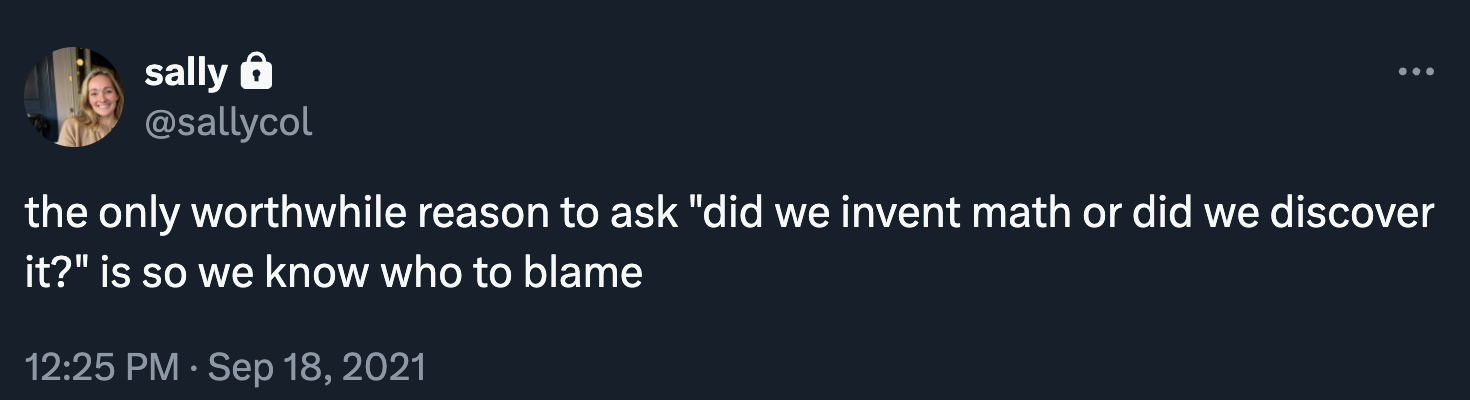
Was it invented or discovered?
This question has been asked millions of times. Seriously.
The answer is probably both!
The question is so popular we can even question the question:
Whatever your take on this question is, Math has proven to be unreasonably effective in the natural sciences.
What are some of its branches?
Math is a big field of study. Here’s how Wikipedia breaks it down (this is just one way, and it’s not going to please everyone):
| Branch | Topics |
|---|---|
| Foundations | Philosophy of Mathematics • Mathematical Logic • Information Theory • Set Theory • Type Theory • Category Theory |
| Algebra | Abstract • Boolean • Clifford • Commutative • Elementary • Field Theory • Group Theory • Homological • Lie • Linear • Multilinear • Ring Theory • Universal |
| Analysis | Calculus • Real Analysis • Complex Analysis • Hypercomplex Analysis • Differential Equations • Functional Analysis • Harmonic Analysis • Measure Theory |
| Discrete | Combinatorics • Discrete Geometry • Graph Theory • Matroid Theory • Order Theory |
| Geometry | Algebraic • Affine • Analytic • Arithmetic • Complex • Computational • Convex • Differential • Discrete • Euclidean • Finite • Information • Projective |
| Number Theory | Algebraic • Analytic • Arithmetic • Diophantine Geometry |
| Topology | General • Algebraic • Differential • Geometric • Homotopy Theory • Knot Theory |
| Applied | Control theory • Operations Research • Probability • Statistics • Game Theory |
| Computational | Computer Science • Theory of Computation • Computational Complexity • Numerical Analysis • Optimization • Computer Algebra |
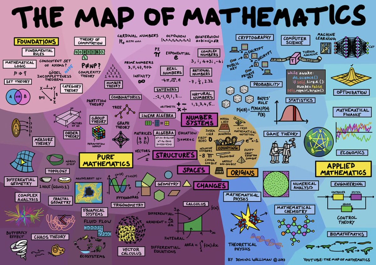
Another organization of topics can be found at Quanta Magazine’s Map of Mathematics. There’s also a cool Map of Mathematics video by Dominic Walliman, from which this poster can be found:
What are Foundations?
We want to put math on a solid foundation so we know that we are not talking nonsense.
If we can reduce everything down to a few very basic concepts and rules that people can agree upon, then show how to carefully and systematically derive all of mathematics from them, building things up in a way everyone can agree is valid, we can have confidence that mathematics does what it is supposed to do.
Whether you believe philosophically that this is possible or not doesn’t matter for now. What matters is putting in the effort to build a foundation and learning from the effort. Honestly, some fascinating discoveries and useful inventions have come from past work in foundations.
Why study Foundations?
Good question! Many mathematicians don’t pursue a deep understanding of the foundations of math because they don’t need it in their daily work. But the field turns out to be really useful for computation, theoretical computer science, formal verification of program correctness (used in computer security), and proving complex theorems with the aid of a computer. In other words, it’s important for computer science, particularly in the study of programming languages.
And actually, there is some mind-blowing stuff here.
What is this page about?
This page is a light and incomplete sketch of topics within the area of the foundations of mathematics, with an eye toward showing that mathematical objects (tuples, sets, functions, numbers, and so on) can be rigorously defined and manipulated according to precise rules. The topics here are chosen because they are useful in theoretical computer science.
A Note About NotationMathematical reasoning benefits from concise, symbolic notation. It wasn’t always this way—until the 17th century or so math was mainly done in prose. Today we have some widely accepted notation for mathematical ideas, but there is still a surprising amount of variation. In fact, you are free to choose your own notation, as long as you are consistent.
Foundational Theories
There are many theories within mathematics. But there are three kinds of theories that can be viewed as providing a foundation for (all of) math: set theories, type theories, and category theories.
See the Wikipedia page on Foundations of Mathematics and the SEP article on Philosophy of Mathematics for a history of the subject.
Oversimplifying a bit, here’s a bit about these three theories (or technically, theory families):
| Set Theory | Type Theory | Category Theory | |
|---|---|---|---|
| Philosophy and Approach | Math is about classification of objects by arranging them in sets. Set theory requires logic (generally a classical one) to already exist. | Math is about manipulating objects according to the types they inhabit. Logic emerges from the theory. Usually constructive in nature (though classical type theories do exist). | Math is about structures and the relationships between them, without worrying about internal details. |
| Key Features | Sets are built up from smaller sets, with rules to avoid paradoxes. Generally, everything is a set, which is both a strength and a weakness. | Terms have types. Types can depend on other types as well as on terms. Propositions are types. Proofs are programs. | Categories have objects and morphisms (arrows or relationships). Functors map between categories. Commutative diagrams are used a lot. |
| Concepts | Elements, membership, subsets, power sets, tuples, sequences, partitions, relations, equivalence relations, orders, cardinality. | Types, terms, inductive types, sums ($+$), products ($\times$), dependent types ($\Pi$ and $\Sigma$), propositions as types, proofs as programs, equality types, universes. | Objects, morphisms, functors, natural transformations, limits, colimits, adjunctions, monads, categories, monoids, topoi. |
| Characteristic Notation | $x \in S$ means $x$ is an element of set $S$. | $x : A$ means the term $x$ is of type $A$. | $X \xrightarrow{f} Y$ means $f$ is a morphism from category $X$ to category $Y$. |
| Applications | Used everywhere—most mathematicians are familiar with much of it. | Computer science, formal verification, proof assistants. | Abstract algebra, topology, geometry, mathematical logic. |
| Exemplars | Some set theories are: ZF and ZFC, NBG, NF and NFU, MK, KP, CST. | Some type theories are: Simply-Typed $\lambda$ calculus, MLTT, System F, DTT, CoC, HoTT. | Some category theories are: ETCS, Topos Theory, Abelian, Monoidal. |
Math and LogicMath and logic are related, but not the same thing. Mathematicians do quite a lot of logic. If interested, I have more extensive notes that get into logic in more detail, with coverage of non-bivalent, intuitionistic, paraconsistent, fuzzy, non-monotonic, and a bunch of other types of logic. They get into metalogical notions of soundness and completeness, too.
Mathematical Objects
Mathematics is concerned with objects and the relationships between them. Before creating a foundational theory, we should take an inventory of the kinds of things that humans work with in mathematics. Then we can start to think about how all of the objects can be encoded with primitive notions. In no particular order, here’s an incomplete sampling of useful mathematical objects:
Booleans Numbers Tuples Sets Relations Functions Sequences Structures Lists Characters Strings Maps Graphs Vectors Matrices Tensors
Different theories construct objects in different ways.
The Set Theory Approach
Most set theories reduce everything to one foundational notion, the set. A set is a (possibly empty) collection of elements, which are themselves sets, constructed in such a way as to avoid nonsense collections.
Let’s begin with notation:
- $x \in A$ is defined to mean $x$ is an element of $A$.
- $x \notin A$ sugars $\neg(x \in A)$, and is read “$x$ is not an element of $A$.”
- $A \subseteq B$ sugars $\forall x. x \in A \supset x \in B$, and is read “$A$ is a subset of $B$.”
There is a lot of notation in Set Theory, so more sugar will be warranted. We’ll be using:
$\begin{array}{lcl} \forall x \in A. P & \textrm{to sugar} & \forall x.\, x \in A \supset P \\ \exists x \in A. P & \textrm{to sugar} & \exists x.\, x \in A \land P \\ \forall x\,y \in A. P & \textrm{to sugar} & \forall x. \forall y.\, x \in A \land y \in A \supset P \\ \exists x\,y \in A. P & \textrm{to sugar} & \exists x. \exists y.\, x \in A \land y \in A \land P \\ \end{array}$
Here are the axioms of ZFC set theory:
We haven’t defined functions yet, but thinking in terms of functions makes the axiom a bit easier to understand. We’ll go deeper into this in class to understand how the intuitive notion of a function is captured by the axiom.
Unlike the other axioms, this one is philosophically controversial. It asserts the existence of a choice function without telling you how to construct one—and for infinite (especially uncountable) collections of sets, there may be no way to describe such a function explicitly. You're just allowed to assume it exists.
Now we know what sets are. To have Set Theory as a foundation for mathematics, we need to be able to encode every mathematical object as a set. But how? Here are some encodings people have invented:
- Natural Numbers
- $0 = \varnothing$
$1 = \{0\} = \{\varnothing\}$
$2 = \{0, 1\} = \{\varnothing,\{\varnothing\}\}$
$3 = \{0,1,2\} = \{\varnothing,\{\varnothing\},\{\varnothing,\{\varnothing\}\}\}$
$4 = \{0,1,2,3\}$
...
$n = \{0,1,2,\ldots,n-1\}$
... - Booleans
- $\textsf{false} = 0$
$\textsf{true} = 1$ - Ordered Pairs
- $(a, b) = \{\{a\}, \{a, b\}\}$
- Tuples
- Ordered pairs that “nest” to the right
- Relations
- Sets of ordered pairs
- Functions and Maps
- Relations in which each left element is unique
- Structures
- Custom arrangements of elements often with tags that carry meaning in a given context
- Sequences
- Functions from $\{0, 1, \ldots n\}$
- Lists
- Nested pairs in which the innermost pair has the form $(x, \varnothing)$
- Characters
- Natural numbers (interpreted as code points)
- Strings
- Lists of characters
- Integers
- Sets of all pairs of natural numbers $(a, b)$ with the same difference $a - b$
- Rational Numbers
- Sets of all pairs of integers $(a, b)$ with $b \neq 0$ with the same quotient $\frac{a}{b}$
- Real Numbers
- Sets of rational numbers with an upper bound but no lower bound that contain all rational numbers less than the upper bound
Details will come later. For now, simply appreciate that everything does seem to be encodable with sets, which is why Set Theory has become so effective and popular.
Also keep in mind that many different kinds of objects have the same structural encodings, but their behaviors may be radically different. All we showed above are the structural encodings of various mathematical objects. The following two exercises should help illustrate this point.
UrelementsSome set theories allow for the existence of items that are not sets, but that can be members of sets. They’re called urelements. ZFC explicitly rejects these because the foundations are easier without them, and they don’t really add any expressive power.
Other Set TheoriesZFC is just one of many set theories. They all resolve the paradoxes arising from being too loose with what is and is not a set, particularly Russell’s Paradox, in different ways. Some theories make self-containing sets impossible to write. NF allows such sets but gets around the root problem with stratification. NBG distinguishes sets and classes.
The Type Theory Approach
Type Theory doesn’t go as deep into making all objects one kind of thing, but does something much more convenient. It allows you to bring into existence whatever objects you need, as long as you give them each a type and construct them carefully. You do this by defining rules that exhaustively specify the inhabitants of a type.
Our first type:
$$ \dfrac{}{\textsf{true}\!: \textsf{Bool}} \quad\quad\quad \dfrac{}{\textsf{false}\!: \textsf{Bool}} $$This states that the type $\textsf{Bool}$ is inhabited by exactly two values, $\textsf{true}$ and $\textsf{false}$. No more, no less. We have created two things. And a type.
Now here is the type of natural numbers:
$$ \dfrac{}{0\!: \textsf{Nat}} \quad\quad\quad \dfrac{n\!: \textsf{Nat}}{\textsf{s}\,n\!: \textsf{Nat}} $$This says “(1) $0$ is a natural number, (2) For any natural number $n$, $\mathsf{s\,}n$ is a natural number, and (3) nothing else is a natural number.” So the type of natural numbers is inhabited by $0$, $\mathsf{s\,}0$, $\mathsf{s\,s\,}0$, $\mathsf{s\,s\,s\,}0$, $\mathsf{s\,s\,s\,s\,}0$, and so on. We’ll write these as $0$, $1$, $2$, $3$, $4$, and so on. These abbreviations should be familiar to you.
Now for the integers:
$$ \dfrac{n\!: \textsf{Nat}}{\textsf{pos}\,n\!: \textsf{Int}} \quad\quad\quad \dfrac{n\!: \textsf{Nat}}{\textsf{neg}\,n\!: \textsf{Int}} $$So the type of integers is inhabited by $\mathsf{pos\,}0$, $\mathsf{neg\,}0$, $\mathsf{pos\,s\,}0$, $\mathsf{neg\,s\,}0$, $\mathsf{pos\,s\,s\,}0$, $\mathsf{neg\,s\,s\,}0$, and so on. We’ll abbreviate these as $0$, $-1$, $1$, $-2$, $2$, $-3$, and so on. But what, then, is the type of $3$? We need to figure it out from context, or we can write $3_{\textsf{Nat}}$ or $3_{\textsf{Int}}$ to be explicit.
Here are the rationals:
$$ \dfrac{n\!: \textsf{Int} \quad d\!: \textsf{Nat}}{\textsf{rat}\,n\,d\!: \textsf{Rat}} $$So one-third is $\textsf{rat}\,1\,3$, which we can abbreviate as $\frac{1}{3}$.
We can build lots of numeric types that are useful in programming languages, for example $\textsf{Int8}$, $\textsf{Int16}$, $\textsf{Int32}$, $\textsf{Int64}$, $\textsf{Int128}$, $\textsf{UInt8}$, $\textsf{UInt16}$, $\textsf{UInt32}$, $\textsf{UInt64}$, $\textsf{UInt128}$, $\textsf{Float16}$, $\textsf{Float32}$, $\textsf{Float64}$, $\textsf{Float128}$, $\textsf{Complex64}$, $\textsf{Complex128}$, and so on. Some might require a lot of rules, but they can be defined in principle.
We can make up more types for ourselves. Here is one for primary colors:
$$ \dfrac{}{\textsf{red}\!: \textsf{PrimaryColor}} \quad\quad\quad \dfrac{}{\textsf{green}\!: \textsf{PrimaryColor}} \quad\quad\quad \dfrac{}{\textsf{blue}\!: \textsf{PrimaryColor}} $$You can define the type $\textsf{Unicode}$ whose inhabitants are, you guessed it, the characters of Unicode. That’d be a lot of rules! But it is indeed definable, as there are a finite number of such characters.
Now here is a type for some simple two-dimensional shapes:
$$ \dfrac{r\!: \textsf{Float64}}{\textsf{circle}\,r\!: \textsf{Shape}} \quad\quad\quad \dfrac{w\!: \textsf{Float64}\quad h\!: \textsf{Float64}}{\textsf{rectangle}\,w\,h\!: \textsf{Shape}} \quad\quad\quad \dfrac{a\!: \textsf{Float64}\quad b\!: \textsf{Float64} \quad c\!: \textsf{Float64}}{\textsf{triangle}\,a\,b\,c\!: \textsf{Shape}} $$The idea is that $\mathsf{circle}\,5.0$ is a circle with radius 5.
Objects can have rather complex structure, if you define the types recursively. Here’s the type “list of elements of type $t$” which we will write $t^*$:
$$ \dfrac{}{[\,]\!: t^*} \quad\quad\quad \dfrac{x\!: t \quad y\!: t^*}{(x :: y)\!: t^*} $$We will write ${[x]}$ for $(x\,\textbf{::}\,[\,])$, ${[x,y,z]}$ for $(x\,\textbf{::}\,(y\,\textbf{::}\,(z\,\textbf{::}\,[\,])))$, and so on. For an empty list, we would need to rely on context to infer its type, or be explicit by writing, for example, $[\,]_\textsf{Int*}$.
Imagine what the type $\textsf{Unicode}^*$ is. Got it? That’s right! We’ll use the abbreviation $\textsf{String}$ for this type. This makes programmers happy.
Now let’s do “option of type $t$” which we will write $t\texttt{?}$:
$$ \dfrac{}{\textsf{none}\!: t\texttt{?}} \quad\quad \dfrac{x\!:t}{\textsf{some}\;x\!: t\texttt{?}} $$We thus have $\textsf{some}\:3\!:\mathsf{Nat}\texttt{?}$ and $\textsf{some}\:(-3,T)\!:(\mathsf{Int \times Bool})\texttt{?}$. When writing $\textsf{none}$, we must rely on context to know which type is being referred to, or you can use subscripts to be explicit, e.g., $\mathsf{none_{Int?}}$.
Here is a type for “binary trees of type $t$”:
There’s a type called $\textsf{Void}$ that has no inhabitants. So there are no constructors.
Just as in Set Theory, there are rules we have to follow to make sure we are not constructing nonsense types. We’ll cover this in detail in our notes on Type Theory.
| Type | Constructors |
|---|---|
| $\textsf{Bool}$ | $\textsf{true}$, $\textsf{false}$ |
| $\textsf{Nat}$ | $0$, $\textsf{s}$ |
| $\textsf{Int}$ | $\textsf{pos}$, $\textsf{neg}$ |
| $\textsf{Rat}$ | $\textsf{rat}$ |
| $\textsf{PrimaryColor}$ | $\textsf{red}$, $\textsf{green}$, $\textsf{blue}$ |
| $\textsf{Shape}$ | $\textsf{circle}$, $\textsf{square}$, $\textsf{triangle}$ |
| $t^*$ | $\texttt{[]}$, $\textsf{::}$ |
| $t\textsf{?}$ | $\textsf{none}$, $\textsf{some}$ |
| $\textsf{Bintree}\lt\!t\!\gt$ | $\textsf{empty}$, $\textsf{node}$ |
| $\textsf{Void}$ | — |
Tuples
Objects such as $()$, $(21,F)$, $(a,a,b,a,b,a,b,b)$, or $(do, re, mi, fa, so, la, ti, do)$ are called tuples. The elements of a tuple are ordered. Given a tuple $t$, you access the $i$th element with the notation $\:t\!\downarrow\!i$.
Please note that $(a,(a,a))$ is not the same thing as $((a,a),a)$.
Tuples in Type Theory
In Type Theory, tuples are built from pairs, whose first element has type $t_1$ and the second has type $t_2$. The type of such pairs is the product type $t_1 \times t_2$:
As a convention, we’ll take $\times$ to be right-associative, so $t_1 \times t_2 \times t_3$ is exactly $t_1 \times (t_2 \times t_3)$, and, correspondingly, $(a,b,c)$ sugars $(a,(b,c))$.
In general, $(a_1, \ldots, a_n)$ sugars $(a_1, (a_2, (\ldots, (a_{n-1}, a_n)\ldots)))$ and is called an $n$-tuple. Its length is $n$.Strictly speaking, under this construction, genuine (nested-pair) tuples have at least $2$ elements. We can extend our linguistic convention to speak of a $1$-tuple as an element itself, i.e., $a = (a)$; and the (yes, THE) $0$-tuple is a special value $()$, with its own type called Unit:
Tuples can be concatenated. If $t_1$ is an $m$-tuple and $t_2$ is an $n$-tuple then $t_1 • t_2$ is an $(m+n)$-tuple:
$$(a_1, \ldots, a_m) • (b_1, \ldots, b_n) = (a_1, \ldots, a_m, b_1, \ldots, b_n)$$We will allow the concatenation operator to work with $0$-tuples and $1$-tuples as well, so $(a,b) • c = (a,b,c)$, $a • b = (a,b)$, and $a • () = a$.
Tuples in Set Theory
We saw earlier that tuples, in Set Theory, are encoded like so: $(a,b) = \{\{a\}, \{a,b\}\}$. This has some rather odd consequences, such as $\{5\} \in (5,3)$ but $\{3\} \not\in (5,3)$,which we ignore in practice. Such oddities are a natural result of building everything from sets. One need only worry about the encoding when dealing with foundations; in practice, tuples can be treated as tuples.
Just as in Type Theory, we will build tuples from pairs. First, a definition. The set of all pairs $(a, b)$ whose first element comes from $A$ and the second from $B$ will be denoted $A \times B$. We can define it as:
$$A \times B =_{\small{\textrm{def}}} \{ z \in \mathcal{P}(\mathcal{P}(A \cup B)) \mid \exists a \in A. \exists b \in B. z = (a, b) \}$$Again, this is just an encoding. You may sometimes see folks write:
However, this is not legal, since the left-hand side of the $\mid$ should be an expression of the form $x \in S$ where $S$ is an existing set (of which we are trying to make a subset from), but this set should be...$S$ itself—the set they are trying to define. However, once $A \times B$ is properly defined, it can be used as a set that can be subsetted. Furthermore, we can pattern match on the left-hand side tuple pattern, so we can eventually get concise notation such as:
$$\{(a, b) \in A \times B \mid a = b\}$$for:
$$\{z \in A \times B \mid \exists a. \exists b. z = (a, b) \land a = b\}$$As in Type Theory, we take the set-theoretic $\times$ to be right-associative, so $A_1 \times A_2 \times \ldots \times A_n$ means $A_1 \times (A_2 \times (\ldots \times A_n)\ldots)$, and $(a_1, \ldots, a_n)$ sugars $(a_1, (a_2, (\ldots, (a_{n-1}, a_n)\ldots)))$. The convenient idea of the $0$-tuple and $1$-tuple from Type Theory carries over to Set Theory. The unit object $()$ is encoded as $\varnothing$.
Sets
A set, in practice, is an unordered collection of unique elements. We denote sets by enumerating their elements or using the filtering notation we introduced above in our discussion of the axiom of separation. Depending on context, we can sometimes get quite informal and use prose, as long as there is a way to recover necessary precision.
Crisp and Fuzzy SetsWhat does it mean to be a member? It can vary.
- For crisp sets, you’re either in or you’re out. No in-between. This is the most common kind of set.
- For fuzzy sets, membership can be partial. For example, you might be 0.8 in the set of tall people.
These notes will only cover crisp sets.
Notation
Set Theory as a foundation uses very few symbols. To make things more convenient, we will expand our language with some additional notation. Let’s first recall what we’ve seen so far:
The various axioms we saw above (particularly separation) allow us to make some very convenient definitions:
AMBIGUOUS NOTATION ALERTThe notation $A^n$ is horribly overloaded! When $A$ is a plain old set, the notation indicates tuple construction. When $A$ is a relation, the notation indicates repeated composition of the relation with itself. When $A$ is an alphabet, the notation indicates the set of strings with a given length. When $A$ is a language, the notation indicates sets of strings made by concatenating strings from $A$ a given number of times.
In each of these cases, the value of $A^n$ is completely different!
Context is crucial to understanding the meaning. Ambiguity is very common in math.
Some Set Theorems
Assuming you already know first-order classical logic, you can use the definitions above to prove some interesting theorems about sets. The following are theorems in any of the major set theories (ZFC, NFU, etc.), with all free variables implicitly universally quantified:
Disjointness and Partitions
Sometimes we want to separate out the elements of a set into non-overlapping groups. Two concepts are useful here.
$A$ and $B$ are disjoint iff $A \cap B = \varnothing$
$\Pi = \{P_1, P_2, \ldots, P_n\} \subseteq \mathcal{P}(A)$ is a partition of $A$ iff:
- $\varnothing \notin \Pi$
- $\forall x\:i\:j. (x \in P_i \land i \neq j) \supset x \notin P_j$
- $\bigcup \Pi = A$
Relations
A relation is a subset of a cross product. That’s it. That’s the whole definition.
For the relation $R \subseteq A \times B$, we say $A$ is the domain and $B$ is the codomain. If $(a,b) \in R$ we write $aRb$. The inverse $R^{-1} \subseteq B \times A$ is $\{(b,a) \mid aRb\}$.
Here is the definition of the less-than relation on natural numbers in set theory:
Note that because a relation is a subset of $A \times B$, the set of all relations over $A$ and $B$ is $\mathcal{P}(A \times B)$.
For $R \subseteq A \times A$ we define:
- $R$ is reflexive iff $\forall a. aRa$
- $R$ is irreflexive (a.k.a anti-reflexive) iff $\forall a. \neg aRa$
- $R$ is symmetric iff $\forall a\:b. aRb \supset bRa$
- $R$ is asymmetric iff $\forall a\:b. aRb \supset \neg bRa$
- $R$ is antisymmetric iff $\forall a\:b. aRb \land bRa \supset a=b$
- $R$ is transitive iff $\forall a\:b\:c. aRb \land bRc \supset aRc$
- $R$ is total iff $\forall a\:b. aRb \vee bRa$
More definitions:
- $R$ is an equivalence relation iff it is reflexive, symmetric, and transitive
- $R$ is a partial order iff it is reflexive, antisymmetric, and transitive
- $R$ is a total order iff it is antisymmetric, transitive, and total
If $R \subseteq A \times B$ and $S \subseteq B \times C$ then the composition of $R$ and $S$ is $S \circ R$ = $\{(a,c) \mid \exists b. aRb \land bSc\}$.
Even though relations are sets, the superscript notation on relations means something different than it does for regular sets. This seems infuriating until you finally come to terms with the fact that that math notation is very contextual and changes depending on what you are talking about. Anyway, here is what the superscripts mean for relations:
Those definitions imply $R^2 = R \circ R$, $R^3 = R \circ R \circ R$, and so on.
These forms turn out to be very useful in computation theories, as we frequently use relations that represent a single computation step, so the * form of the relation will mean any number of steps.
AMBIGUOUS NOTATION ALERTThe expression $R^2$ is ambiguous: since a relation is a set, $R^2$ could mean $R \times R$, but most people use it to mean $R \circ R$. You really need to supply context when using ambiguous notation.
Functions
A function maps an input to an output, such that given any input (called the argument), you get the same output every time you apply the function.
In Type Theory, a function maps every inhabitant of the input type, called the domain to a value in the output type, called the codomain. If a function $f$ has domain $t_1$ and codomain $t_2$, then $f$ inhabits the type $t_1 \to t_2$. To apply or invoke the function $f$ on argument $a$, we write $f\,a$ or $f(a)$. To represent a function explicitly, we write:
$$\lambda x_t. e$$where $x$ is the argument of the function, $t$ is the type of the argument, and $e$ is the expression that computes the output based on $x$. Usually the output type is inferrable, but if it is not, writing $(\lambda x. e)\!: t_1\to t_2$ is totally fine.
We specify functions by showing how to compute the output for each possible input. We base this off the constructors of the type. Remember the Boolean type? It has only two constructors, $\textsf{true}$ and $\textsf{false}$. So boolean negation is the function:
$$ \lambda x_{\textsf{Bool}}. \textsf{match}\;x\;\textsf{when}\;\textsf{true} \rightarrow \textsf{false}\;\textsf{when} \;\textsf{false} \rightarrow \textsf{true}$$The type of natural numbers we saw above has two constructors: $0$ and $\textsf{s}$. The “is zero” function on natural numbers is:
$$ \lambda x_{\textsf{Nat}}. \textsf{match}\;x\;\textsf{when}\;0 \rightarrow \textsf{true}\;\textsf{when} \;\textsf{s}\,n \rightarrow \textsf{false}$$And the “plus two” function on natural numbers is:
$$ \lambda x_{\textsf{Nat}}. \textsf{match}\;x\;\textsf{when}\;0 \rightarrow \textsf{s}\,\textsf{s}\,0\;\textsf{when} \;\textsf{s}\,n \rightarrow \textsf{s}\,\textsf{s}\,\textsf{s}\,n$$Sometimes the match cases collapse into one, as in the plus two function, which can be written more succinctly as:
$$ \lambda x_{\textsf{Nat}}. \textsf{s}\,\textsf{s}\,n$$We often want to give names to functions to make them easier to refer to. We can write, for example:
$$ \textsf{isZero} =_{\small{\textrm{def}}} \lambda x_{\textsf{Nat}}. \textsf{match}\;x\;\textsf{when}\;0 \rightarrow \textsf{true}\;\textsf{when} \;\textsf{s}\,n \rightarrow \textsf{false}$$But it is more common to write a definition by cases. Here are the three functions we have seen so far:
$\begin{array}{l} \textsf{not}\!: \textsf{Bool} \rightarrow \textsf{Bool} \\ \textsf{not}\;\textsf{true} = \textsf{false} \\ \textsf{not}\;\textsf{false} = \textsf{true} \end{array}$
$\begin{array}{l} \textsf{isZero}\!: \textsf{Nat} \rightarrow \textsf{Bool} \\ \textsf{isZero}\;0 = \textsf{true} \\ \textsf{isZero}\;(\textsf{s}\,n) = \textsf{false} \end{array}$
$\begin{array}{l} \textsf{plusTwo}\!: \textsf{Nat} \rightarrow \textsf{Nat} \\ \textsf{plusTwo}\;0 = \textsf{s}\,\textsf{s}\,0 \\ \textsf{plusTwo}\;(\textsf{s}\,n) = \textsf{s}\,\textsf{s}\,\textsf{s}\,n \end{array}$
Parameters can be tuples:
$\begin{array}{l} \textsf{and}\!:\textsf{Bool} \times \textsf{Bool} \rightarrow \textsf{Bool} \\ \textsf{and}\;(\textsf{true}, \textsf{true}) = \textsf{true} \\ \textsf{and}\;(\textsf{true}, \textsf{false}) = \textsf{false} \\ \textsf{and}\;(\textsf{false}, \textsf{true}) = \textsf{false} \\ \textsf{and}\;(\textsf{false}, \textsf{false}) = \textsf{false} \end{array}$
But since functions are objects, we can do without tuple parameters, and define functions more simply. Study this:
$\begin{array}{l} \textsf{and}\!: \textsf{Bool} \rightarrow (\textsf{Bool} \rightarrow \textsf{Bool}) \\ \textsf{and}\;\textsf{true} = \lambda x_{\textsf{Bool}}.\,x \\ \textsf{and}\;\textsf{false} = \lambda x_{\textsf{Bool}}.\,\textsf{false} \end{array}$
Got it? Then this should make sense:
$\begin{array}{l} \textsf{or}\!: \textsf{Bool} \rightarrow (\textsf{Bool} \rightarrow \textsf{Bool}) \\ \textsf{or}\;\textsf{true} = \lambda x_{\textsf{Bool}}.\,\textsf{true} \\ \textsf{or}\;\textsf{false} = \lambda x_{\textsf{Bool}}.\,x \end{array}$
We can simplify a little more, squeezing out the lambda expressions:
$\begin{array}{l} \textsf{and}\!: \textsf{Bool} \rightarrow (\textsf{Bool} \rightarrow \textsf{Bool}) \\ \textsf{and}\;\textsf{true}\;x = x \\ \textsf{and}\;\textsf{false}\;x = \textsf{false} \end{array}$
$\begin{array}{l} \textsf{or}\!: \textsf{Bool} \rightarrow (\textsf{Bool} \rightarrow \textsf{Bool}) \\ \textsf{or}\;\textsf{true}\;x = \textsf{true} \\ \textsf{or}\;\textsf{false}\;x = x \end{array}$
Here is how to add natural numbers. Make sure to study the definition carefully. It is recursive, but well-defined since the recursive portion operates on a component that is structurally smaller than the argument of the clause in which it appears:
$\begin{array}{l} \textsf{plus}\!: \textsf{Nat} \rightarrow \textsf{Nat} \rightarrow \textsf{Nat} \\ \textsf{plus}\;0\;m = m \\ \textsf{plus}\;(\textsf{s}\,n)\;m = \textsf{s}\,(\textsf{plus}\;n\;m) \end{array}$
Multiplication:
$\begin{array}{l} \textsf{times}\!: \textsf{Nat} \rightarrow \textsf{Nat} \rightarrow \textsf{Nat} \\ \textsf{times}\;0\;m = 0 \\ \textsf{times}\;(\textsf{s}\,n)\;m = \textsf{plus}\;m\;(\textsf{times}\;n\;m) \end{array}$
Exponentiation:
$\begin{array}{l} \textsf{exp}\!: \textsf{Nat} \rightarrow \textsf{Nat} \rightarrow \textsf{Nat} \\ \textsf{exp}\;0\;m = 1 \\ \textsf{exp}\;(\textsf{s}\,n)\;m = \textsf{times}\;m\;(\textsf{exp}\;n\;m) \end{array}$
Less Than:
$\begin{array}{l} \textsf{lt}\!: \textsf{Nat} \rightarrow \textsf{Nat} \rightarrow \textsf{Bool} \\ \textsf{lt}\;0\;0 = \textsf{false} \\ \textsf{lt}\;0\;(\textsf{s}\,m) = \textsf{true} \\ \textsf{lt}\;(\textsf{s}\,n)\;0 = \textsf{false} \\ \textsf{lt}\;(\textsf{s}\,n)\;(\textsf{s}\,m) = \textsf{lt}\;n\;m \end{array}$
And here is something remarkably useful:
$\begin{array}{l} \textsf{cond}\!: \textsf{Bool} \rightarrow t \rightarrow t \rightarrow t \\ \textsf{cond}\;\textsf{true}\;x\;y = x \\ \textsf{cond}\;\textsf{false}\;x\;y = y \end{array}$
Ok hold up! It’s time to introduce some notation to make things a bit more familiar. From now on, we’re going to write:
$\begin{array}{lll} \neg b & \text{for} & \textsf{not}\;b \\ a \land b & \text{for} & \textsf{and}\;a\;b \\ a \lor b & \text{for} & \textsf{or}\;a\;b \\ \textsf{if}\;b\;\textsf{then}\;x\;\textsf{else}\;y & \text{for} & \textsf{cond}\;b\;x\;y \\ n + 1 & \text{for} & \textsf{s}\;n \\ m + n & \text{for} & \textsf{plus}\;n\;m \\ m \times n & \text{for} & \textsf{times}\;n\;m \\ m^n & \text{for} & \textsf{exp}\;n\;m \\ n \lt m & \text{for} & \textsf{lt}\;n\;m \\ \textsf{let}\;x = e\;\textsf{in}\;e' & \text{for} & (\lambda x.\,e')\;e \end{array}$
Heck we’ll even write $xy$ for $x \times y$ except when it makes things too confusing.
We can in principle define more numeric types and more arithmetic and logical operations. We won’t do so here, but feel free to do so. It can be fun! This can take us to places where things start to look convenient, and familiar. Here are a couple functions using the $\textsf{Shape}$ type defined earlier:
$\begin{array}{l} \textsf{area}\!:\textsf{Shape} \rightarrow \textsf{Float64} \\ \textsf{area}\;(\textsf{Circle}\;r) = \pi r^2 \\ \textsf{area}\;(\textsf{Rectangle}\;w\;h) = wh \\ \textsf{area}\;(\textsf{Triangle}\;a\;b\;c) = \textsf{let}\;s = \frac{a + b + c}{2} \;\textsf{in}\; \sqrt{s(s-a)(s-b)(s-c)} \\ \end{array}$
$\begin{array}{l} \textsf{perimeter}\!:\textsf{Shape} \rightarrow \textsf{Float64} \\ \textsf{perimeter}\;(\textsf{Circle}\;r) = 2 \pi r \\ \textsf{perimeter}\;(\textsf{Rectangle}\;w\;h) = 2 (w + h) \\ \textsf{perimeter}\;(\textsf{Triangle}\;a\;b\;c) = a + b + c \\ \end{array}$
When defining functions by cases, the type annotation on the function name gives us enough context to infer the types of the clauses in the definition. When the function stands alone, explicit type annotations are often necessary, especially when using operators that look the same across many types:
Sometimes, annotating only the parameters is sufficient, since the types of the bodies are often inferrable:
Polymorphic Functions
Here’s a fun one. What is the type of $\lambda f. \lambda x. f(f(x))$? Well, $(\textsf{Int} \rightarrow \textsf{Int}) \rightarrow \textsf{Int} \rightarrow \textsf{Int}$ works.
But so does $(\textsf{Real} \rightarrow \textsf{Real}) \rightarrow \textsf{Real} \rightarrow \textsf{Real}$. And so does $(\textsf{Bool} \rightarrow \textsf{Bool}) \rightarrow \textsf{Bool} \rightarrow \textsf{Bool}$. And so on. We can generalize the type by introducing type variables.
The type is $\forall \alpha. (\alpha \rightarrow \alpha) \rightarrow \alpha \rightarrow \alpha$. You don’t have to write the $\forall$ though. But it is a nice way to say, “you can substitute any type you like for the type variable $\alpha$.” We say this function is polymorphic.
Did you notice that the function $\textsf{cond}$ that we saw above was also polymorphic?
Functions are Sets in Set Theory
In set theory, where everything is a set, even functions, a function $f \subseteq A \times B$ is just a relation in which every element of $A$ appears exactly once as the first element of a pair in $f$. That’s all it is.
If $f$ is a function and $(a,b) \in f$ we write $f a = b$, or $f(a) = b$, and say $b$ is the value of $f$ at $a$. The range of $f$ is $\{b \mid \exists a. b = f a\}$.
The set of all functions from $A$ to $B$ is denoted $A \rightarrow B$. Looks just like the type theory notation! You might also see $B^A$ used for this set.
Since functions are relations and therefore sets, we can write them in set notation, but it’s totally fine to use the $\lambda$ notation from Type Theory. It’s fine to share notation between theories! Even though the notation is similar, remember that in Type Theory, the domain and codomain are types, while in Set Theory, the domain and range are sets. The distinction matters, even though the notation blurs it somewhat.
A reminder: we sometimes we don’t make the domain or range explicit if we can infer them from context.
Sets are Functions in Type Theory
So how about this? If you start with Type Theory and you want sets, you can represent a set as a function returning a boolean value. Return $\textsf{true}$ if the input should be in the set and $\textsf{false}$ otherwise.
This means that:
- The set $\{ x \in \mathbb{N} \mid x \bmod 2 = 0\}$ is the function $\lambda x_{\textsf{Nat}}. x \bmod 2 = 0$
- The set $\{ x \mid e \}$ is the function $\lambda x. e$
- The expression $x \in A$ is just $A\,x$. (Do you see why?)
Yeah, sets feel like they just exist. They are just there. They feel static, ontological. But functions are always in motion, computing things, answering questions. They feel dynamic, phenomenological.
More Sugar!
A few forms make $\lambda$-expressions easier to read. The first is the amazing let-notation that we saw earlier, but did not really dive into. Here it is again, because it is so useful and is used all the time:
- For example: $\;\mathsf{let}\;x=3\;\mathsf{in}\;x+5$ evaluates to $8$
- Because: $\;\mathsf{let}\;x=3\;\mathsf{in}\;x+5$ is the same as $(\lambda x . x+5)(3)$
- In general: $\;\mathsf{let}\;x=e\;\mathsf{in}\;e'$ is the same as $(\lambda x . e')(e)$
Where-notation is a close relative of let-notation:
- For example: $\;x+5\;\mathsf{where}\;x=3$ evaluates to $8$
- Because: $\;x+5\;\mathsf{where}\;x=3$ is the same as $(\lambda x . x+5)(3)$
- In general: $\;e'\;\mathsf{where}\;x=e$ is the same as $(\lambda x . e')(e)$
If-notation:
- $\mathsf{if}\;b\;\mathsf{then}\;x\;\mathsf{else}\;y = \textsf{match}\;b\;\textsf{when}\;\textsf{true} \rightarrow x\;\textsf{when}\;\textsf{false} \rightarrow y$
Equivalently:
- $\mathsf{if}\;b\;\mathsf{then}\;x\;\mathsf{else}\;y = \begin{cases} x & b = \textsf{true} \\ y & b = \textsf{false}\end{cases}$
Substitution:
- $f[a \mapsto b] = \lambda x. \mathsf{if}\;x=a\;\mathsf{then}\;b\;\mathsf{else}\;f(x)$
Function iteration:
- $f^0(x) = x$
- $f^1(x) = f(x)$
- $f^2(x) = f(f(x))$
- $f^3(x) = f(f(f(x)))$
- ...
- $f^{n+1}(x) = f(f^n(x))$
AMBIGUOUS NOTATION ALERTMany mathematicians purposefully blur the distinction between $\sin^2\theta$ and $(\sin \theta)^2$, leaving you, the poor reader, to figure out what they mean by context. It can be very annoying.
It appears that for trigonometric functions, people tend to use the iterative form for the power form, but for other functions the iterative form usually means iteration. Maybe?
Don’t worry too much. It’s all a consequence of the fact that everyone is allowed to invent their own notation. Just remember, all things are contextual.
AMBIGUOUS LANGUAGE ALERTIf $f$ is a function, do not say “the function $f(x)$” unless the function $f$, when applied to $x$, actually yields a function. Also do not say things like “the function $n^2$” because $n^2$ is a number. The function you probably have in mind is $\lambda n. n^2$. That doesn’t stop people from abusing the notation, though.
Mathematics is often about communicating ideas, not about absolute precision. Confusing people is part of the fun of math, it seems. Context matters. When something is ambiguous, ask about it.
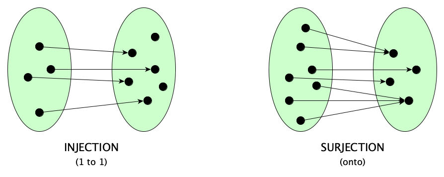
The -jections
Time for more definitions! For $f:\!A \rightarrow B$ (or $f \in A \rightarrow B$ for you set theorists, since the following works the same in both theories):
- $f$ is a surjection (i.e., $f$ maps $A$ onto $B$) iff $\forall b. \exists a. f a = b$
- $f$ is an injection (i.e., $f$ maps $A$ one-to-one to $B$) iff $\forall a . \forall b. a \neq b \supset f a \neq f b$
- $f$ is a bijection, a.k.a. a one-to-one correspondence iff $f$ is a surjection and an injection
If $f$ is a bijection from $A$ to $B$, then:
- $f^{-1}$ is a bijection from $B$ to $A$
- $\forall a. f^{-1}(f\,a) = a$
- $\forall b . f(f^{-1}\,b) = b$
Partial Functions
We defined a function as a relation where every element of the domain appears exactly once as the first element of a pair. If we relax this to every element of the domain appearing at most once then we have a partial function. Think of a partial function as not being able to compute a value for every element, or one in which the value at some inputs is “undefined.” For emphasis, functions are defined everywhere are called total functions.
The set of all partial functions from $A$ to $B$ is denoted $A \rightharpoonup B$.
If $f \in A \rightharpoonup B$ then:
- $f \in C \rightarrow B$ for some $C \subseteq A$, where $C$ is precisely the set of elements from $A$ at which $f$ is defined.
- $f \in A \rightarrow B \cup \{\bot_B\}$, where $\bot_B$ is a representation of the undefined value in $B$.
The type subscript on $\bot_B$ is often omitted in practice and inferred from context.
Partial functions are useful in computer science because they allow us to model programs that might not terminate or might throw an error. However, the modern approach in programming languages is that for functions that may fail, we use total functions whose codomain is a sum or union type combining expected return values and error values. For functions that never terminate, well, partial functions are fine.
Sequences
A sequence is an ordered list of elements indexed by natural numbers, and written $\langle a_0, a_1, a_2, \dots, a_{n-1} \rangle$. The length of the sequence is $n$.
In Set Theory, a sequence is a partial function from the natural numbers $\mathbb{N}$ to some set $A$, where the function is defined for the first $n$ natural numbers and undefined thereafter. To get the element at position $i$ in sequence $s$, we simply evaluate $s(i)$.
Alternatively, a sequence can be encoded as a total function with domain $\{ 0, 1, \ldots, n-1\}.$
Lists
We already saw how to define lists in Type Theory; here’s the definition of the type “list of elements of type $t$” again:
$$ \dfrac{}{[\,]\!: t^*} \quad\quad\quad \dfrac{x\!: t \quad y\!: t^*}{(x :: y)\!: t^*} $$Recall that we get the conventional notation by writing ${[x]}$ for $(x\,\textbf{::}\,[\,])$, ${[x,y,z]}$ for $(x\,\textbf{::}\,(y\,\textbf{::}\,(z\,\textbf{::}\,[\,])))$, and so on.
To define lists in Set Theory, we can use a similar inductive approach as in Type Theory. The empty list is represented by $\varnothing$, and a non-empty list is represented as an ordered pair whose first element is the head of the list and the second element is the tail (which is itself a list). So the list $[3,8,5]$ would be represented as $(3, (8, (5, \varnothing)))$.
Strings
Strings in set theory are encoded as lists of characters, where a character is an element of a set known as an alphabet. An example of an alphabet is the set $\textsf{Unicode}$. The set theory representation of the string $hi$ is $(\texttt{LATIN SMALL LETTER H}, (\texttt{LATIN SMALL LETTER I}, \varnothing))$.
In Type Theory, the type of strings is simply $\textsf{Unicode}^*$.
The context surrounding strings is so vast, we have a separate page of notes on the topic. It is part of a much larger theory of language and computation, which we will explore in detail later in the course.
Maps
Sometimes it’s convenient to think of partial functions as maps where the inputs are the keys and the outputs are the values. When we do, we tweak the notation a bit. Here’s a partial function, $m \in \textsf{Unicode}^* \rightharpoonup \mathbb{N}$:
$(\lambda s. \bot)[\texttt{a} \mapsto 1][\texttt{b} \mapsto 2][\texttt{c} \mapsto 3]$
The function substitution notation is perfect here, as it says that the value at every input is $\bot$ unless explicitly overwritten. But we said above that functions are just sets. Which set is this? We can say it’s this:
$\{ (\texttt{a}, 1), (\texttt{b}, 2), (\texttt{c}, 3) \} \cup \{ (s, \bot) \mid s \in \textsf{Unicode}^* \setminus \{\texttt{a}, \texttt{b}, \texttt{c}\} \}$
It’s a bit hard to read, though, so in these cases, we do better writing the function in map notation:
$\{ \texttt{a}\!: 1, \texttt{b}\!: 2, \texttt{c}\!: 3 \}$
We will consider the latter just syntactic sugar for the former, rather than defining maps as a primitive type. So for this particular map, we have:
Also, because maps are just functions, the substitution notation works for them too. If $m$ is the map above, we can write things like $m[\texttt{d} \mapsto 4]$ for the map just like $m$ with the additional key-value pair mapping $d$ to $4$, and $m[\texttt{b} \mapsto 0]$ for the map like $m$ except $\texttt{b}$ now maps to $0$.
Numbers
Numbers are so useful. We use them to count, measure, order, compare, and so much more.
Some people love numbers. Some numbers have a lot of fascinating properties. Some are interesting philosophically and recreationally. If you like numbers, or even if you think you don’t, browse Robert Munafo’s pages on notable numbers. You’ll probably like it!
Kinds of Numbers
Numbers are classified by how we use them. Here is a small sampling:
| Type | Concept | What it tells us |
|---|---|---|
| Cardinal Numbers | Quantity | How many discrete items |
| Ordinal Numbers | Sequence | The position of something in an ordering |
| Scalar Numbers | Magnitude | How much (continuous quantity) of something there is |
| Coordinate Numbers | Location | Numbers that represent a position in space |
| Vector Numbers | Direction and Magnitude | Which way and how far |
| Nominal Numbers | Identification | A convenient label |
Here is another way to classify numbers:
| Kind | Symbol | Informal Description |
|---|---|---|
| Natural Numbers | $\mathbb{N}$ | $\{0, 1, 2, 3, \ldots\}$ |
| Integers | $\mathbb{Z}$ | $\{\ldots, -3, -2, -1, 0, 1, 2, 3, \ldots\}$ |
| Rational Numbers | $\mathbb{Q}$ | $\{\frac{a}{b} \mid a, b \in \mathbb{Z} \land b \neq 0\}$ |
| Real Numbers | $\mathbb{R}$ | (See the Wikipedia article) |
| Complex Numbers | $\mathbb{C}$ | Has 2 real components, written ($a+bi$) |
| Quaternions | $\mathbb{H}$ | Has 4 real components, written ($a+bi+cj+dk$) |
| Octonions | $\mathbb{O}$ | 8 real components, with units $e_0 ... e_7$ |
| Sedenions | $\mathbb{S}$ | 16 real components |
There are more! Did you know about algebraic vs. transcendental numbers? This amazing diagram by Keith Enevoldsen shows how they fit in (up to the complex numbers, at least):
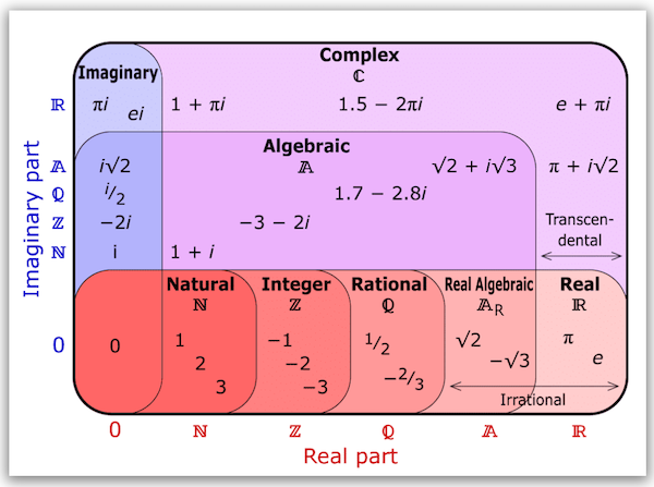
We can even slip in a couple more categories, Computable and Describable, which are very useful in computer science theory. Here is where they land in the real numbers hierarchy:
That’s right! There are real numbers that we can describe but not compute. There are real numbers that exist but that we can’t even describe. This makes computer science (and math) interesting. How we know that we have proper containment at each level of this hierarchy is a little beyond the scope of these notes, but something you should research and internalize at some point.
$\Omega$The number $\Omega$ in the diagram above is Chaitin’s constant, a number we can describe but not compute. It’s not the same $\Omega$ as the mathematically inconsistent, self-contradictory “absolute infinity” from the Vi Hart video later in these notes.
Things get interesting when you go beyond the reals. What isn’t “real” by the way? Imaginary perhaps? Not a good name, as Jade shows:
Perhaps if they got a better name, the video would have had a different title.
Operations
Before we get to foundational definitions of numbers, let’s look at some basic operations we can perform with them (informally, of course).
For natural numbers:
- Addition: $x^{(1)}y = x + y = \underbrace{\:s\: \ldots \:s\:}_{y}\;x$
- Multiplication: $x^{(2)}y = x \times y = \underbrace{\:x + x + \ldots + x\:}_{y}$
- Exponentiation: $x^{(3)}y = x \uparrow y = \underbrace{\:x \times x \times \ldots \times x\:}_{y}$
- Tetration: $x^{(4)}y = x \uparrow\uparrow y = \underbrace{\:x \uparrow x \uparrow \ldots \uparrow x\:}_{y}$ (also called hyper4 or power-tower)
- Pentation: $x^{(5)}y = x \uparrow\uparrow\uparrow y = \underbrace{\:x \uparrow\uparrow x \uparrow\uparrow \ldots \uparrow\uparrow x\:}_{y}$
- And on and on....
Addition, multiplication, and exponentiation work for real numbers too. There are also inverses:
- Subtraction: $x - y$ = the $z$ such that $y + z = x$
- Division: $x \div y$ = the $z$ such that $y \times z = x$
- Logarithm: $\log_y(x)$ = the $z$ such that $y^z = x$
- And there are “inverses” of the operators beyond exponentiation as well
Got all that? Do you have a good sense of these numbers and operations? You should. Being numerically literate, with a good feel for numbers gives you agency in the world, become less likely to be taken advantage of, and helps you become a better citizen. Watch Vi Hart’s piece which should give you a feel for what having feels about numbers entails:
Also important:
- The floor of a real number $x$, denoted $\lfloor x \rfloor$, is the largest integer less than or equal to $x$.
- The ceiling of a real number $x$, denoted $\lceil x \rceil$, is the smallest integer greater than or equal to $x$.
Defining Numbers
Earlier, we saw the how to define, in Type Theory, the types natural numbers, integers, and rationals. How can these be encoded in Set Theory? We already saw the set of natural numbers—$\mathbb{N}$—the set that exists by the Axiom of Infinity:
$$ \begin{array}{lcl} \mathbb{N} & = & \{ \varnothing, \{\varnothing\}, \{\varnothing, \{\varnothing\}\}, \{\varnothing, \{\varnothing\}, \{\varnothing, \{\varnothing\}\}\}, \ldots \} \\ & = & \{0, 1, 2, 3, \dots\} \end{array} $$The intuitive approach to encoding integers and rational numbers in set theory goes like this:
- An integer is encoded as a set of pairs $(a, b)$ from $\mathbb{N} \times \mathbb{N}$, such that, say, the integer $3$ is encoded as $\{ (3,0), (4,1), (5,2), \dots \}$ and the integer $-2$ is encoded as $\{ (0,2), (1,3), (2,4), \dots \}$. The set of all integers is called $\mathbb{Z}$.
- A rational number is encoded as a set of pairs $(a, b)$ from $\mathbb{Z} \times (\mathbb{Z} \setminus \{0\})$, such that, say, the rational number $\frac{3}{4}$ is encoded as $\{ (3,4), (6,8), (9,12), \dots \}$ and the rational number $-\frac{2}{5}$ is encoded as $\{ (-2,5), (-4,10), (-6,15), \dots \}$. The set of all rational numbers is called $\mathbb{Q}$.
But to make this formal, we need to define what we mean by addition and multiplication for natural numbers within set theory.
Here is the successor function on natural numbers in set theory:
$$ S =_{\small{\textrm{def}}} \{ (x,y) \in \mathbb{N} \times \mathbb{N} \mid y = x \cup \{x\} \} $$Now addition on natural numbers is the smallest relation that satisfies the properties of addition, which should look familiar to you from our definition in Type Theory above:
$$ + =_{\small{\textrm{def}}} \bigcap \left\{ R \in \mathcal{P}((\mathbb{N} \times \mathbb{N}) \times \mathbb{N}) \ \middle|\ \begin{array}{l} (\forall m \in \mathbb{N}. \, (m, 0)\,R\, m) \; \land \\ (\forall m, n, k \in \mathbb{N}. \, (m, n)\,R\, k \supset (m, S(n))\,R\, S(k)) \end{array} \right\} $$Now we can formally define the sets of integers and rational numbers:
Real Numbers are pretty wild, and require some cleverness to define set-theoretically. The trick is to model it as a set of all rational numbers less than the number we are defining—more precisely, a bounded, downward-closed (if $x$ is in the set and $y$ is a rational number less than $x$, then $y$ is also in the set) set of rationals that is neither $\varnothing$ or $\mathbb{Q}$ itself, called a Dedekind Cut. Specific examples are:
The set of all real numbers:
The “missing” arithmetic operations on naturals, rationals, and reals are beyond the scope of these notes, but worth studying.
Cardinal Numbers
A cardinal number tells us how many of something there are. In particular, it helps us count how many items there are in a set. The quantity of elements in a set is called the cardinality of the set. The cardinality of set $A$ is denoted $|A|$ and obeys these axioms:
- $|A| = |B|$ iff there exists a bijection between $A$ and $B$. That is, for each element in $A$ there is a matching value in $B$ and vice-versa.
- $|A| \leq |B|$ iff there exists an injection from $A$ to $B$. That is, for each element of $A$ there is a matching element in $B$, but not necessarily vice-versa.
- $|A| < |B|$ iff $|A| \leq |B|$ and $|A| \neq |B|$
Did you notice something about bijections? They are important! They tell us when two sets are the same size, without having to count them.
Matching is more fundamental than counting.
Think about thisMatching is more fundamental than counting. Imagine yourself without words for what we now call numbers. You could still come up with ideas of greater than or less than, and allocate resources, and even trade.
Counting is an advanced concept!
If there exists a bijection between a set $A$ and the set $\{1, 2, ... k\}$ for some natural number $k \geq 0$, we say that $A$ is finite and, since the number of elements in $\{1, 2, ... k\}$ is $k$, we have $|A| = k$.
What about $\mathbb{N}$? We can’t find a bijection between that and $\{1, 2, ... k\}$ for any natural number $k$. That set is not finite—it is infinite. So what is its cardinality? Someone once declared it to be $\aleph_0$ and this stuck. $\aleph_0$ a cardinal number. Not a natural number, but definitely a cardinal, because it tells you how many of something there is.
We can make a bijection between the set of even numbers and the set of natural numbers using the function $\lambda n_{\small{\mathbb{N}}}. 2n$. So the set of even numbers has the same cardinality as the set of natural numbers. It too has a cardinality of $\aleph_0$.
An interesting thing about $\mathbb{N}$ is that you can list, enumerate, or count them—yes it would take forever, but you could do it in principle. The is so significant that we have a definition:
A set $A$ is countable (a.k.a. listable) iff $A$ is finite or $|A| = \aleph_0$. $\mathbb{N}$ is countable by definition. We saw that the even natural numbers are countable. So is $\mathbb{Z}$, because $\lambda n.(\textsf{if}\;\textit{even}(n)\;\textsf{then}\;\frac{-n}{2}\;\textsf{else}\;\frac{n+1}{2})$ is a bijection between $\mathbb{N}$ and $\mathbb{Z}$.
$\mathbb{N} \times \mathbb{N}$ is countable, too:
  (0,0)
  (0,1)   (1,0)
  (0,2)   (1,1)   (2,0)
  (0,3)   (1,2)   (2,1)   (3,0)
  (0,4)   (1,3)   (2,2)   (3,1)   (4,0)
  (0,5)   (1,4)   (2,3)   (3,2)   (4,1)   (5,0)
  ...
By a similar argument, $\mathbb{Q}$, $\mathbb{N}^i$, and any countable union of countable sets are all countable.
But the set of real numbers is associated with a bigger infinity. We prove this with a technique known as diagonalization, which basically says that no matter how you try to list all real numbers, you can always construct a new real number that is not on the list.
Here’s a video explanation, together with some additional historical context:
The video shows that there are infinities “larger than” the infinity of the natural numbers. That is, there are cardinal numbers much greater than $\aleph_0$. Such sets are called uncountable. There are infinitely many larger and larger and larger infinities. You can show this by making power sets repeatedly. Why? Because Cantor’s theorem works for both finite (obviously) and infinite sets:
Cantor’s Theorem: For any set $A$, $|A| \lt |\mathcal{P}(A)|$. Proof: Clearly $|A| \leq |\mathcal{P}(A)|$, so we only have to show $|A| \neq |\mathcal{P}(A)|$. Proceed by contradiction. Assume $|A| = |\mathcal{P}(A)|$, which means there is a function $g$ mapping $A$ onto $\mathcal{P}(A)$. Consider $Y = \{x \mid x \in A \land x \notin g(x)\}$. Since $g$ is an onto function, there must exist a value $y \in A$ such that $g(y)=Y$. If we assume $y \in Y$ then by definition means that $y \notin Y$. But if we assume $y \notin Y$, then that means $y \in Y$. This is a contradiction, so the assumption that a surjectve $g$ exist cannot hold. Therefore $|A| \neq |\mathcal{P}(A)|$. Slay.
Diagonalization againCantor’s theorem uses the same diagonalization technique as the proof that $|\mathbb{N}| \lt |\mathbb{R}|$.
Similar arguments to this proof of Cantor’s theorem show that the following sets are uncountable:
- $\{x \mid x \in \mathbb{R} \land 0 \lt x \lt 1\}$
- $\mathbb{N} \rightarrow \mathbb{N}$
Fun fact. Okay so $\{x \mid x \in \mathbb{R} \land 0 \lt x \lt 1\}$ is uncountable. But is its cardinality equal to, or strictly less than, $\mathbb{R}$ itself? Turns out it’s equal! The bijection you are looking for is: $\lambda x. \frac{1}{\pi}tan^{-1}x + \frac{1}{2}$ is a bijection to $<0,1>$.
The continuum is a pretty mind-blowing concept.
The fact that $\mathbb{N}\rightarrow\mathbb{N}$ is uncountable means that there are functions for which no computer program can be written to solve, because programs are strings of symbols from a finite alphabet of characters (e.g., Unicode) and thus there are only a countably infinite number of them. Similarly, the fact that there are real numbers that we cannot describe is true because descriptions are themselves finite strings in some language.
The continuum is a pretty mind-blowing concept.
Alternate DefinitionsRather than defining finite sets as those can have a bijection with $\{1, 2, \ldots k\}$ for natural number $k$ and infinite sets as sets that are not finite, others prefer these definitions:
A set is infinite iff there is a bijection between it and a proper subset of itself. A set is finite iff it is not infinite.
Ordinal Numbers
An ordinal number gives the position of something in an ordered sequence. While cardinal numbers are called, in English, zero, one, two, three, and so on, ordinal numbers are called first, second, third, and so on.
Ordinals are interesting because they give us new kinds of infinities. This Vsauce video has a good explanation with good visuals:
Big Numbers
Robert Munafo has another catalog of numbers, his Large Numbers pages, which you absolutely don’t want to miss. It includes not only large numbers, but the transfinite ordinals.
Seriously, don’t miss it!
Have ten hours to spare? This will take you through large finite numbers only, but in doing so, will give you a sense that thinking that infinity is not a big deal isn’t really accurate. Though easy to describe, it’s so far beyond direct experience. You just can’t.
If you want to become immersed and well-versed in this stuff, start at the Googology Wiki. Have fun!
Even More Numbers
There are so many more kinds of numbers.
Here’s Vi Hart again, taking you far beyond anything we’ve yet seen:
So many types of numbers in this video: cardinals in set theory, surreals in game theory, supernaturals in field theory, ordinal spaces in topology, Hilbert spaces in analysis and quantum physics, and more.
Arrays of Numbers
We’ll close with something not exactly foundational, but important enough to talk about their representation and behavior: arrays of numbers, such as vectors, matrices, and tensors.
Structurally, a vector is a tuple that contains numbers. Behaviorally, while a tuple just kind of sits there, a vector comes with associated operations obeying the laws of a vector space such as vector addition and scalar multiplication.
Structurally, a matrix is a two-dimensional array of numbers. Behaviorally, a matrix comes with associated operations obeying the laws of matrix algebra such as matrix addition and matrix multiplication.
Structurally, a tensor is a multi-dimensional array of numbers. Behaviorally, a tensor comes with associated operations obeying certain laws.
Details are outside of the scope of this page.
Math and Computation
Much of mathematics is aided by the use of computers. Computers speed up time, allowing us to think previously unthinkable thoughts. Computers make science and mathematics qualitatively different. Computers augment and amplify human thought. In math, complex proofs can be found, or at least checked, by an automated proof assistant. Generally, these proof assistants are based on Type Theory, not Set Theory, for various reasons (many taken from these slides by Sergey Goncharov):
- In Type Theory, functions are primitive. They are not just special kinds of sets of pairs. Functions compute things, and thus feel dynamic. Why look at them like static relations?
- Set Theory purports to be simpler, in that it has fewer basic notions, as in everything is a set. But this really isn’t the case, as the axioms of Set Theory are really complex and few people know them all. The axioms are arguably arbitrary and don’t help much in finding proofs. Set Theory is just too theoretical.
- Set Theory’s “everything is a set” approach is actually too simple. We want to distinguish tuples and functions and relations and numbers. Mathematicians naturally think in terms of different types of objects. Why treat them all as sets? This leads to silliness like $2 \in 3$ and $\pi \cap \mathbb{R}$.
- In Set Theory, logic and objects come first, then we use sets to group the objects. In type theory, types come first, then we construct objects to inhabit the types, and logic emerges. Thus Type Theory does not decouple logic from the objects it defines the way Set Theory does.
- Most type theories are constructive! There’s no excluded middle, for one thing. To prove existentials, you have to supply a witness. To prove disjunctions, you have to show one of the disjuncts. Computation feels constructive. In contrast, most set theories are classical.
- Set Theory’s underlying logic has debatable principles such as the Excluded Middle, the Axiom of Choice, and Impredicativity, which get in the way of automation.
Hello? Category Theory?Yes, we made a decision to focus on Set Theory and Type Theory only. Two theories are enough to get you started on the foundational aspects of mathematics. Category Theory is important, but it can be explored after gaining a solid understanding of Set Theory and Type Theory.
Math and Logic
Remember how we started with the observation that Logic is a prerequisite for Set Theory, but Logic emerges from Type Theory? Perhaps this means Type Theory is more fundamental? Maybe. But it does indicate something: there must be a deep connection between Logic and Type Theory.
We won’t cover it all right now, but will leave you with something to think about. Here is the type inference rule that tells us the type of the output of a function application:
That looks like Modus Ponens in logic. Is that a coincidence or an interesting correspondence?
And the inference rule for inferring the type of a pair is:
Can’t you just feel logical conjunction here?
This is just a small part of the Curry-Howard correspondence, which we’ll see when we cover Type Theory in depth.
Beyond Foundations
This page is focused on foundations. But there’s much more to math that is useful in computer science. You might want to check out:
- Counting principles (pigeonhole, addition, multiplication)
- Permutations
- Combinations
- Probability, for which you really need to see the amazing Seeing Theory: A Visual Introduction to Probability and Statistics
- Recurrence Relations
- Type Theory
- Category Theory
- Information Theory
- Algebraic Structures
- Linear Algebra
- Geometry
- Topology
- Analysis
- Formal Proofs
- Numerical Analysis
- Optimization
- Graph Theory
- Number Theory
- Algebra
Does Math Describe the World?
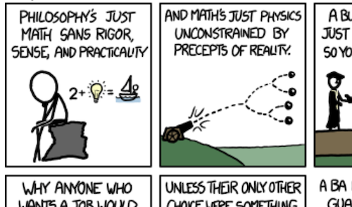
Did you watch the Vsauce video above? Kind of cool how Michael says we can do math that isn’t science and just invent things that we declare to be true, like transfinite infinities, and yeah, as long as we don’t have contradictions, let’s go. The first two frames of the famous XKCD Every Major’s Terrible has fun with this idea:
Sometimes our inventions do give us good models. Cohl Furey explains it in two minutes:
Intrigued? Watch her entire Division Algebras And the Standard Model playlist. Or checkout this article on her work.
Recall Practice
Here are some questions useful for your spaced repetition learning. Many of the answers are not found on this page. Some will have popped up in lecture. Others will require you to do your own research.
- What are some things that are reasoned about within mathematics? Quantity, structure, change, chance, causality, and space.
- Mathematic reasoning involves finding abstract ________________ and constructing ________________ of real and imaginary phenomena. patterns, models.
- Was math invented or discovered? Probably both.
- What are some of the main branches within mathematics? Foundations, algebra, analysis, discrete, geometry, number theory, topology, applied mathematics, and computational mathematics.
- What are three theories that claim to be able to formalize “all of mathematics”? Set Theory;
Type Theory;
Category Theory. - What are the characteristic notations of set, type, and category theory? $x \in A$
$x : A$
$X \xrightarrow{f} Y$ - What is perhaps the main difference between set theory and type theory? In set theory, everything is a set. In type theory, types come first, and objects are constructed to inhabit the types.
- What are some of the foundational mathematical objects? Booleans, numbers, tuples, characters, strings, sequences, relations, functions, sets, vectors, matrices, tensors, maps, graphs.
- What are the rules for inhabiting the type of natural numbers? $\dfrac{}{0\!:\textsf{nat}}$$\dfrac{n\!:\textsf{nat}}{sn\!:\textsf{nat}}$
- What does a tuple look like?
$(a, b, c)$- What is $(10, 20, 30)\downarrow 1$?
$20$- What kind of a type do tuples belong to?
A product type.- What is the unit type?
The type with only one inhabitant, $()$.- What is $(2, 8, 3) \bullet (5, 1)$?
$(2, 8, 3, 5, 1)$- Why are sets so effective at formalizing mathematics?
A set expresses the very fundamental notion of an object having a property.- How do sets differ from tuples?
Sets are unordered and do not contain duplicates.- What is the difference between a crisp set and a fuzzy set?
A crisp set is a set where an element is either in the set or not. A fuzzy set is a set where an element can be partially in the set.- How do we denote that $x$ is a member of the set $A$?
$x \in A$- Why isn’t $\{ x \mid x \not\in x \}$ considered a set?
Considering it a set ruins everything because if it were a set, assuming it was a member of itself would imply it was not and assuming it was not a member of itself would imply that it was.- How is set subtraction $A \setminus B$ defined?
$\{x \mid x \in A \land x \notin B\}$- What is the difference between $A-B$ and $A \setminus B$?
Nothing, they are the same.- What is the difference between $A \setminus B$ and $A \vartriangle B$?
The first is the set of all elements in $A$ but not in $B$. The second, the symmetric difference, is the set of elements that are in exactly one of $A$ or $B$.- What is $\mathcal{P}(\{a,b,c\})$?
$\{\varnothing, \{a\}, \{b\}, \{c\}, \{a,b\}, \{a,c\}, \{b,c\}, \{a,b,c\} \}$- What is $\bigcup \{ \mathbb{Q}, \mathbb{R}, \mathbb{N}\}$?
$\mathbb{R}$- What is $\bigcap \{ \mathbb{Q}, \mathbb{R}, \mathbb{N}\}$?
$\mathbb{N}$- What is $\varnothing \times \varnothing$?
$\varnothing$- What is $\{1,2\}^*$?
$\{(), (1), (2), (1,1), (1,2), (2,1), (2,2), (1,1,1), (1,1,2), (1,2,1), (1,2,2), (2,1,1), \ldots \}$- What is $\{1, 2\}^0$?
$\{ () \}$- What are the distinct partitions of $\{ a, b \}$?
- $\{ \{a\}, \{b\} \}$
- $\{ \{a,b\} \}$
- What are the distinct partitions of $\{ a, b, c \}$?
- $\{ \{a\}, \{b\}, \{c\} \}$
- $\{ \{a,b\}, \{c\} \}$
- $\{ \{a,c\}, \{b\} \}$
- $\{ \{b,c\}, \{a\} \}$
- $\{ \{a,b,c\} \}$
- Are the set of all even integers and the set of all prime numbers disjoint?
No, they share the number $2$.- Given a relation $R$ defined as a subset of $A \times B$, what are $A$ and $B$ called?
The domain and codomain of $R$.- How do we denote the set of all relations over $A$ and $B$?
$\mathcal{P}(A \times B)$- What is the inverse of the relation $\{(1, 2), (3, 4)\}$?
$\{(2, 1), (4, 3)\}$- Give an example of a relation over $\{a, b, c\}$ that is neither reflexive nor irreflexive.
$\{(a, a), (b, c)\}$ is not reflexive because it does not contain $(b, b)$, and it is not irreflexive because it does contain $(a, a)$.- What is the difference between “asymmetric” and “antisymmetric”?
An asymmetric relation can never have a member of the form $(x,x)$, but an antisymmetric relation can.- What three properties characterize a partial order?
Reflexivity, antisymmetry, transitivity.- Let $R_1 = \{(3,1),(9,8),(2,5)\}$ and $R_2 = \{(8,8),(10,2),(1,7)\}$. What is $R_1 \circ R_2$?
$\{ (10,5) \}$- Let $R = \{ (3, 5), (5, 8), (1, 2), (8, 1) \}$. What are $R^2$ and $R^3$?
$R^2 = \{ (3, 8), (5, 1), (8, 2) \}$
$R^3 = \{ (3, 1), (5, 2) \}$- How do we denote the type of a function from $A$ to $B$?
$A \rightarrow B$- What is another way to show the types on the expression $(\lambda x. x \bmod 2 = 0)\!:(\mathsf{nat \rightarrow bool})$
$\lambda x_{\small \textsf{nat}}. x \bmod 2 = 0$, is sufficient, because we can infer the body has type $\textsf{bool}$.- What is the type of $\lambda x. x$?
$\alpha \rightarrow \alpha$- How do we denote the set of all functions from $A$ to $B$?
$A \rightarrow B$- How do we represent the set $\{ (x, y) \mid x \in \mathbb{N} \land y \in \mathbb{N} \land x > y \}$ as a function in Type Theory?
$\lambda (x, y)_{\small \mathsf{nat \times nat}}. x > y$- Is $\{ (x, y) \mid x \in \mathbb{Z} \land y \in \mathbb{Z} \land x = y^2 \}$ considered a function in Set Theory?
No, because both $(1, 1)$ and $(1, -1)$ are in the relation, so that’s two distinct pairs with the same left element.- The set $\mathbb{Z} \times \{ 0 \}$ is a function. Write it in lambda notation.
$\lambda x_{\small \textsf{int}}. 0$- How do you write let $x = 8$ in $2^x - 1$ without the “let”?
$(\lambda x. 2^x - 1)(8)$- How do you write $(\lambda x. x + 3)(5)$ in where-notation?
$x + 3\;\textsf{where}\;x = 5$- The set $\{ (x, y) \mid x \in \mathbb{N} \land \textrm{x is even} \land y = \frac{x}{2} \} \cup \{ (x, y) \mid x \in \mathbb{N} \land \textrm{x is odd} \land y = \frac{3x+1}{2} \}$ is a function. Write it in lambda notation, using an if expression.
$\lambda x_{\small \textsf{nat}}. \textsf{if}\;\textit{even}(x)\;\textsf{then}\;\frac{x}{2}\;\textsf{else}\;\frac{3x+1}{2}$- Suppose $f = \lambda x. x^2$ and $g = \lambda x. x + 3$. What are $f \circ g$ and $g \circ f$?
$f \circ g = \lambda x. (x + 3)^2$
$g \circ f = \lambda x. x^2+3$- Suppose $f = \lambda x. 5x + 2$ and $g = f[1 \mapsto 2]$. What are $g(8)$ and $g(1)$?
$g(8) = 42$
$g(1) = 2$- How do you write the function that maps
"x"to 21,"y"to 8,"z"to 55, and every other input to 0, in both lambda notation and as a map?$(\lambda x. 0)[21/\texttt{"x"}][8/\texttt{"y"}][55/\texttt{"z"}]$
$\{ \texttt{"x"}\!: 21, \texttt{"y"}\!: 8, \texttt{"z"}\!: 55 \}$- Let $f = \lambda x. 3x + 5$. What are $f^{-1}$, $f^0$, $f^1$, and $f^2$?
$f^{-1} = \lambda x. \frac{x-5}{3}$
$f^0 = \lambda x. x$
$f^1 = \lambda x. 3x + 5$
$f^2 = \lambda x. 9x + 20$.- What is an injection?
A function that maps distinct inputs to distinct outputs. Also known as a one-to-one function.- What is a surjection?
A function that maps to every element in the codomain. Also known as an onto function.- What is the difference between a function and a partial function?
A function maps every element of the domain to an element of the codomain. A partial function maps every element of the domain to either zero or one element of the codomain.- How do we denote the set of all functions from $A$ to $B$? All partial functions from $A$ to $B$?
$A \rightarrow B$; $A \rightharpoonup B$- If a partial function $f$ has no value at $x$, what do we say $f(x)$ is?
$\bot$- How to we write the partial function mapping the vowels of the English alphabet to their 1-based position in the alphabet in map-notation?
$\{ \texttt{a}\!: 1, \texttt{e}\!: 5, \texttt{i}\!: 9, \texttt{o}\!: 15, \texttt{u}\!: 21 \}$- What kind of number is this: $3 + 8i - 5j + k$?
A quaternion.- What kind of a number is $2 - 5e_0 * 8e_6$?
An octonion.- What do we call $\uparrow$, $\uparrow\uparrow$, and $\uparrow\uparrow\uparrow$?
Exponentiation, tetration, pentation.- How do you conventionally write $5 \uparrow\uparrow 3$?
$5^{5^5}$- Perform “one-step” in the simplification of $8 \uparrow\uparrow\uparrow 5$. That is, write the expression in terms of the $\uparrow\uparrow$ operator alone.
$8 \uparrow\uparrow\uparrow 5 = 8 \uparrow\uparrow (8 \uparrow\uparrow (8 \uparrow\uparrow (8 \uparrow\uparrow 8)))$- What are the ”inverses” of addition, multiplication, and exponentiation?
Subtraction, division, logarithm.- What is $\log_2 1024$ and why?
$10$, because $2^{10} = 1024$- What is $\log_{2} 0.125$ and why?
$-3$, because $2^{-3} = \frac{1}{2^3} = \frac{1}{8} = 0.125$- What is cardinal number?
A number that tells you how many of something there is.- ________________ is more fundamental than counting.
Matching- What are the cardinalities of $\varnothing$, $\{a, b, c\}$, and $\mathbb{Z}$?
0, 3, $\aleph_0$- What is an infinite set?
A set for which there exists a bijection between it and a proper subset of itself.- What is a countable set?
A set for which there exists a bijection between it and $\mathbb{N}$.- Which of the following sets are countable and which are not: $\mathbb{N}$, $\mathbb{Z}$, $\mathbb{Q}$, $\mathbb{R}$, $\mathbb{C}$?
$\mathbb{N}$, $\mathbb{Z}$, and $\mathbb{Q}$ are countable. $\mathbb{R}$ and $\mathbb{C}$ are uncountable.- What does Cantor’s Theorem say?
For any set $A$, $|A| < |\mathcal{P}(A)|$.- Who is the guy that made that freaking amazing set of web pages on big numbers?
Robert P. Munafo- (From the Cohl Furey video) What branches of physics do the complex numbers and the quaternions, respectively, play a central role in?
Quantum mechanics; Special relativity.Summary
We’ve covered:
- What mathematics is concerned with
- Overview of foundational theories
- Object construction
- Sets
- Functions
- Numbers
- Connections between Math and Computation
- Connections between Math and Logic
- What else is out there in math world
- Philosophical musings about math and reality
- What does a tuple look like?