Turing Machines

The Backstory

History helps a lot! Why do we have Turing Machines? Why do we care? Why are we better knowing about Turing Machines than not knowing them?

Hear the answers in class. We’ll go through 19th century advances in logic, the formalists versus the intuitionists, Hilbert’s Challenges, the need to formalize computation, Gödel’s and Church’s approaches, and how Turing’s view of computation was the most mechanistic (as opposed to logical or mathematical) and influenced by human computers of the day, and how he (Turing) translated all these ideas into simple mathematical constructs that in some real sense....nailed it!

The Basic Idea

Turing looked at computers of his day and asked “What are these people doing?” He thought about it and realized these folks would write something down, think for a bit, write something else or erase something, think some more, write or erase, and so on. They would move from mental state to mental state as they worked, deciding what to do next based on what mental state they were in and what was currently written.

He realized he could capture this process formally and keep the model very simple: instead of a two-dimensional page, a single one-dimensional tape would do, and instead of randomly jumping around, it would be okay to move one cell at a time. Today we picture the machines like this:

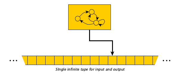
The control portion that defines the operation of the machine is a table that says:

When in state $q$ looking at symbol $\sigma$, (1) optionally write a new symbol, (2) optionally move one cell left or right, and (3) optionally enter a new state $q'$.

The tape starts holding the input with an infinite number of blanks on both sides. (If and) when the machine gets to a state where there is nothing to do at the current symbol, the machine halts.

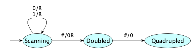
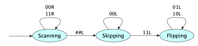
A simple introductory example computation—multiplying a binary number by 4—can be carried out according to the following table:

When in state	Looking at	Perform these actions
Scanning	0	Move right
Scanning	1	Move right
Scanning	#	Print 0, Move right, Go to Doubled state
Doubled	#	Print 0, Go to Quadrupled state

The table is the “Turing Machine.” There is a nice graphical visualization for it, too:

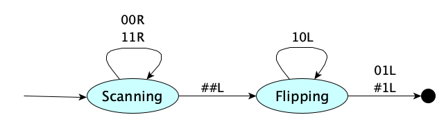
You may notice that “not printing” can be represented with printing the same symbol being read, and “not transitioning” can be represented with going to the same state. “Not moving” can be represented with a stationary move indicator. Tables can then be made more regular, like so:

When in state	Looking at	Print	Move	And go to state
Scanning	0	0	Right	Scanning
Scanning	1	1	Right	Scanning
Scanning	#	0	Right	Doubled
Doubled	#	0	None	Quadrupled

This allows us to dispense with the arrows in our diagrams, marking each transition with a complete triple of (1) input symbol, (2) output symbol, and (3) move direction. Here’s the multiply-by-four machine in this style:

Sometimes, you will see versions of a TM that do not allow stationary moves. So no N’s. Just L’s and R’s only. This can be slightly annoying but it feels simpler to some people. It’s not a problem because you can always simulate a stationary move with two moves in opposite directions.

Here’s the story of the development of the Turing Machine and its impact:

Thirteen Examples

Let’s see some examples before we get formal:

1. Multiply a binary number by 4
2. Floor-divide a binary number by 4
3. Increment an unsigned binary number
4. Two’s complement negation of a binary number
5. Output the string HELLO
6. Determine if a signed binary number is negative
7. Determine if a string is all zeros
8. Determine if a string has exactly three zeros
9. Determine if a string does not contain three consecutive zeros
10. Determine if a binary number is divisible by 3
11. Determine if a string in $\{a,b\}^*$ is a palindrome
12. Recognize the language $\{a^{2^n} \mid n \geq 0\}$
13. Recognize the language $\{a^n b^n \mid n \geq 0\}$

The video uses machines without stationary moves.

More Examples

If the 13 examples in the video were not enough, we have more. We’ll allow stationary moves again.

Even Parity

Given a string of 0s and 1s, we’d like to make the string have an even number of 1s. If it already does, we’ll add a 0; if it doesn’t, we’ll add a 1.

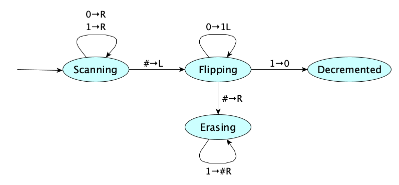
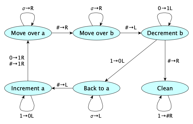
Binary Decrement

Scan to the end of the string. Working backwards, change all 0s to 1s, until you find a 1 to change to 0. If, after the 0s, you don’t find a 1 (but instead hit a blank), you know your input was 0, so it can’t be decremented. In this case, erase all the 1s you just wrote, leaving the tape fully blank to indicate the error.

Reverse a String

This machine reverses any string over the alphabet $\{a, b, c\}$. We’ve introduced the abbreviation $\sigma$ on the left-hand side of a transition to stand for any symbol in the input alphabet $\Sigma$. So $\sigma\to L$ abbreviates three separate rules. It saves space!

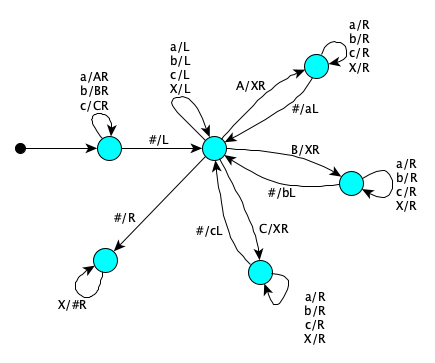
We’ll explain the workings of this machine in class. If you are self-studying, the following sequence of tape snapshots may help:

abbacb
abbacXb
abbaXXbc
abbXXXbca
abXXXXbcab
aXXXXXbcabb
XXXXXXbcabba
      bcabba

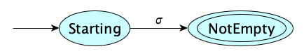
Is Empty?

Initial state is an accept state. Finding any symbol at all transitions to a reject state. You only have to examine the first symbol. As always, we use $\sigma$ to represent any symbol in the alphabet.

Is Nonempty?

Initial state is a reject state. Finding any symbol at all transitions to an accept state. You only have to examine the first symbol. As always, we use $\sigma$ to represent any symbol in the alphabet.

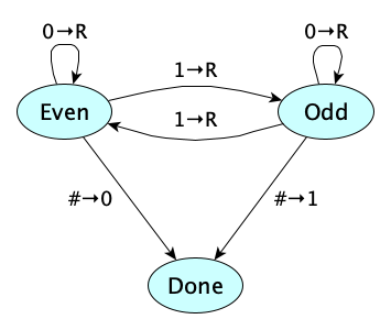
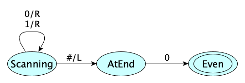
Is Even?

Scan to the end and accept if the last symbol is $0$. Note that if the string is initially empty, you’ll get stuck in the $\textsf{AtEnd}$ state and reject.

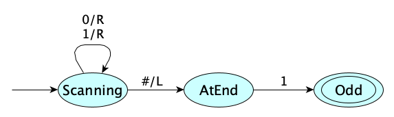
Is Odd?

Scan to the end and accept if the last symbol is $1$. Note that if the string is initially empty, you’ll get stuck in the $\textsf{AtEnd}$ state and reject.

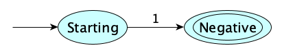
Is (a signed binary integer) Negative?

The string just has to start with a $1$. That’s all.

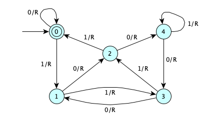
Is Divisible by 5?

Take the empty string to be 0. Read the binary string from left to right. Whenever you see a zero, your current number goes from $n$ to $2n$. Whenever your see a 1, your number increases to $2n+1$. Keep track of the current number modulo 5. You accept if you finish with a number whose value mod 5 is 0.

Binary Addition

This one will be developed and described in class.

But here’s a sample flow for 13+4, in case you want to do some self study:

1101#100
1110#011
1111#010
10000#001
10001#000
10001

Random Dice Roll

This one takes advantage of the fact that when in a state looking at a symbol, you may have more than one action to take.

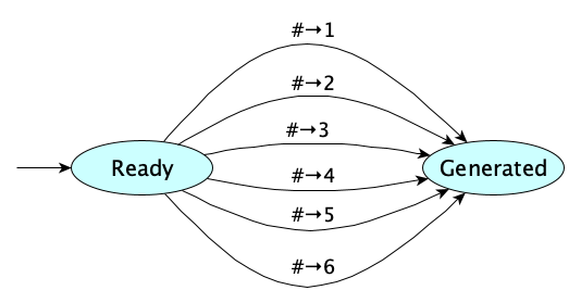
Computing with choices like this is called nondeterminism. A Turing Machine with multiple possible actions for a given state and symbol is called a nondeterministic Turing Machine.

Another Divisible By Four Machine

We can use nondeterminism in recognizers, too. We say that an input is recognized, or decided, by a nondeterministic TM, if there is at least one computation that ends in an accept state. There could be some paths that reject; we only require one that accepts.

So here’s a machine that determines whether its input is divisible by four:

Not very pretty, perhaps.

We’ll go through all the possibilities: $\varepsilon$, $0$, $1$, $00$, $01$, $10$, $11$, $000$, $001$, $010$, $011$, $100$, $101$, $110$, and $111$, $1000$, and so on. We’ll ensure everything divisible by 4 has at least one accept path, and values not divisible by 4 are rejected on all paths.

Even More Examples

Want even more examples? Check out this article with six interesting examples, including:

• Binary addition
• Converting binary to unary
• Converting unary to binary
• Doubling the length of a sequence
• The 4-state busy beaver
• Palindrome detection

Formal Definition

Y’all set for a formal definition?

Remember, when we formalize, we want to go down to the simplest kind of model. That means we will using the variety of machine in which each step always writes a single symbol and always moves either right or left.

Remember, from our earlier notes on Automata Theory that machines can be transducers (produce an output) or recognizers (answer yes or no). We need a separate definition for each.

Here is the definition for a transducing TM:

The recognizing variety can be defined in terms of the transducer:

Recognizers and Deciders

Note that a recognizer just has to answer YES for all strings in the language it is trying to recognize. For strings not in the language, a recognizer may loop forever. If a recognizer always halts with a YES or NO, it is called a decider.

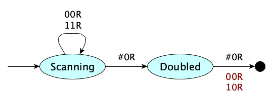
Example. Let’s use the formal definition to describe a Turing Machine that increments a binary number. Here’s the machine as a picture:

and here is the machine as a table:

State	Symbol	Write	Move	Next State
$\textsf{S}$	$0$	0	R	$\textsf{S}$
$\textsf{S}$	$1$	1	R	$\textsf{S}$
$\textsf{S}$	$\#$	$\#$	L	$\textsf{F}$
$\textsf{F}$	$1$	0	L	$\textsf{F}$
$\textsf{F}$	$0$	1	L	$\textsf{I}$
$\textsf{F}$	$\#$	1	L	$\textsf{I}$

Let’s identify the parts. (For simplicity, we’ll use a single character for the state names.) Our machine is $(Q, \Sigma, \Gamma, \#, R, \textsf{S})$ where:

So there you have it. Any Turing Machine is just a mathematical object. Now we can study them formally.

But first, one more piece of notation. For a transducer machine $M$ starting on input string $w$, the output produced by the machine, if it halts, is denoted $M(w)$.

Yep, machines are like functions.

Encoding

There are many ways to succinctly encode (unambiguously) a Turing machine. A common approach lists only the rules, using a single symbol for each state, making the start symbol appear at the beginning of the first rule, and simply inferring the base and tape alphabets. For example:

    S00RS_S11RS_S##LF_F01LI_F#1LI

Since each rule has exactly five symbols, we don’t really need the underscores:

    S00RSS11RSS##LFF01LIF#1LI

Later when we look at deterministic machines, we will see a different encoding.

Given a machine $M$, we generally use $\langle M\rangle$ to refer to its encoding.

The nice thing about encoding machines is that, since the encoding of a machine is just a string, we can provide a machine’s encoding as the input to another machine. So we can make machines that can answer questions about other machines.

But Turing showed there was something else that encodings could lead to. Something really profound.

Universality

In principle, we can build Turing Machines for computing all kinds of functions, such as capitalizing text, finding words in text, computing interest payments, finding documents on the World Wide Web, etc. But functions themselves can be represented in symbols, whether in mathematical notation, plain text Python, or any formalism of your choice. Just a few minutes ago,we saw that the Turing machine to increment a binary number was encoded as S00RSS11RSS##LFF01LIF#1LI.

Turing actually showed something amazing! He defined a machine (call it $U$) such that:

$$ U(\langle M \rangle\texttt{#}x) = M(x) $$

$U$ is a universal machine in the sense that if you give it the encoding of a machine $M$ and some input $x$, it will give you the same output that $M$ would on $x$. It simulates (or emulates or executes or runs, whatever you want to call it) $M$. In fact, $U$ can simulate any machine $M$. So it’s universal.

The idea that only ONE machine was needed to compute all (computable) functions, and not zillions of machines for different kinds of functions, is something we take for granted today, but it was not shown to be true until the 20th century! Really! (As far as anyone knows, that is.) This profound result pretty much changed the world. $U$ is now called the Universal Turing Machine to honor its inventor. Today we build variations of the original $U$. We call them computers.

Stop.

Think about this.

Woah.

Just woah.

This may the most profound idea anyone has ever had about computing.

Are you starting to see why Alan Turing is revered as the founder of computer science?

You can also start reading about Universal Machines at Wikipedia.

Variations on the Turing Machine

Let’s mix things up a bit.

Stationary “Moves”

Instead of having to go left or right at each step, you can also provide to option to stay put. No change to computing power.

$$R \subseteq (Q \times \Gamma) \times (\Gamma \times \{\textsf{L},\textsf{R},\textsf{N}\} \times Q)$$

Here $\textsf{N}$ means stay on the same cell. Think of $\textsf{N}$ as “no move.”

$\varepsilon$-Moves

In the base model, the machine looks at the current symbol and decides what to do next. We can let it just decide to jump to another state without examining the current symbol. Again, no change in computing power.

$$R \subseteq (Q \times (\Gamma \cup \{ \varepsilon \})) \times (\Gamma \times \{\textsf{L},\textsf{R}\} \times Q)$$

Multidimensional Tapes

How about, instead of a tape that is infinite only in the left and right directions, we make a two dimensional tape that can go up and down also?

$$R \subseteq (Q \times \Gamma) \times (\Gamma \times \{\textsf{L},\textsf{R}, \textsf{U}, \textsf{D}\} \times Q)$$

Or a 3-D tape? Or make a machine whose tape is any finite number of dimensions? All good. These extensions do not increase the computing power of the model.

Multiple Tapes

More than one tape? So much more convenient. But you guessed it, no change in computing power.

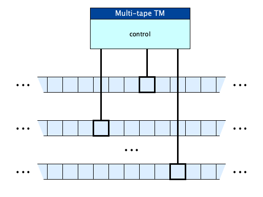
The rule relation for an $n$-tape Turing Machine is simply:

$$R \subseteq (Q \times \Gamma^n) \times ((\Gamma \times \{\textsf{L},\textsf{R}\})^n \times Q)$$

Stack and Queue Tapes

If we restricted our tape memory to act like a queue, we have a Queue Automaton and have no change in computing power. But if our tape was stack-like, we’ve reduced our power: we can no longer compute certain functions (recognize certain languages). But if we had two stacks we are back to full power.

Read-Only and Write-Only and Append-Only Tapes

Restrictions common in multitape machines include prohibiting certain kinds of operations of particular tapes. A read-only tape can only be read, a write-only tape can only be written to, and an append-only tape can only have symbols added at the end.

One-way Infinite Tape

What if the tape had a left-end, and was infinite only to the right? A little messier to program, perhaps, but no change in computing power. With this model, we add a new left-end marker symbol to the tape alphabet (not the input alphabet), and initialize the machine like so:

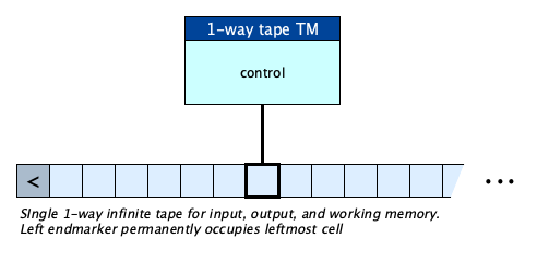
Life without the end marker is not fun. It becomes hard for the machine to know when it has hit the end of the tape. And if it tries to move left, should the machine halt? Or should it just stay in place? The endmarker solves all of these problems.

And there is no change in computational power. A 1-way infinite tape can compute anything a basic Turing Machine can.

To formalize, we add to the basic TM:

and slightly modify the definition of $R$ so that the left marker is only allowed in one cell and can never be overwritten, nor moved left from:

and specify that the machine’s initial configuration has the endmarker followed by the input:

Linear Bounded Automata (LBAs)

What if we bounded the tape on both ends? A Linear Bounded Automaton is a TM with a bounded tape, just big enough to hold the input, and two endmarkers. This is an interesting restriction to place on Turing Machines, since, after all, real machines do have finite memory.

To aid in making a formal definition of an LBA, we introduce two additional special tape symbols, the left-end-marker and the right-end-marker. These symbols can not be overwritten, can not appear anywhere else on the tape, and you cannot move beyond them.

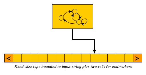
Any change in computing power? It turns out that there is! The computing power is reduced.

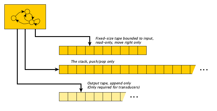
Pushdown Automata (PDAs)

Another restriction that can be placed on a TM is to prevent it from going back and forth—the input can only be read left-to-right until it is exhausted, while allowing a separate “scratch memory” in the form of an ulta-efficient stack, as a second tape. Such a machine is called a push-down automaton (PDA). Transition rules take (1) the current state, (2) optionally the current input symbol, and (3) optionally the stack top, to determine the next state and stack operations. The machine is supposed to exhaust its input and empty its stack. If it gets stuck without a transition with remaining input or a nonempty stack, the machine is said to crash with an error (if a transducer) or reject (if a recognizer).

Transducers are pretty rare in PDA land, but they do exist. They produce output on a third, append-only tape, which is initially empty.

Here is the formal definition of a recognizer PDA:

Pay particular attention to the transition relation. It says: when in state $q$ with the next input symbol $\sigma$ and stack top $\tau$, you consume the input symbol $\sigma$, pop the stack top $\tau$, move to state $q'$, and push $\tau'$ on the stack.

Finite Automata (FAs)

What if we had no memory at all, and we require the whole input to be consumed, one symbol at a time? We’d have something called a Finite Automaton.

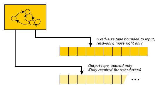
A lot of computations fall into this category.

In a Finite Automaton, the machine must run through the entire input. If it cannot, because it gets stuck in a state with no legal transition, the computation crashes with an error (for a transducer) or immediately rejects (for a recognizer).

Here is the formal definition of a recognizer FA:

Quite a bit easier to define than the general Turing machine!

Random Access

Instead of only moving left, right, or staying in place, what if the machine could jump to any position on the tape directly? This capability is known as random access.

Formally, the transition relation simply becomes: $$R \subseteq (Q \times \Gamma) \times (\Gamma \times \mathbb{Z} \times Q)$$ where the second component of the codomain is an integer representing the position to jump to. We assume the input begins at position 0. Alternatively, this integer can be the number of cells to move relative to the current position (positive to move right, negative to move left, and zero to stay in place).

A random access Turing Machine cannot compute anything more than a regular Turing Machine can, but in some cases it can compute much more efficiently.

Determinism

We’ve defined our machines with a transition relation that could have multiple outgoing transitions from a state for the same configuration. But what if we required the machine to have, for every state, one and only one transition? That is, instead of:

$$ R \subseteq (Q \times \Gamma) \times (\Gamma \times \{\textsf{L}, \textsf{R}\} \times Q) $$

we required $R$ to be a function? Doing so makes the machine deterministic because there is one and only one thing to do at every step. Traditionally, when we move from a relation to a function, we replace $R$ with $\delta$.

Then we can reorient the table to look like this:

	0	1	$\cdots$	#
A
B
C
$\vdots$

But now, the big thing is, since functions have to have an output for every input, we have to expand the codomain so that the machine can stop.

But there are two completely reasonable ways to do this. Neither of which is the right way. We have to look at both.

The Halting Action Variety

One approach is to add a halting action:

$$ \delta : (Q \times \Gamma) \rightarrow (\Gamma \times \{\textsf{L}, \textsf{R}\} \times Q) \cup \{ \textsf{HALT} \} $$

This says: if the machine is in some state $\sigma \in Q$, and currently looking at a symbol $\sigma \in \Gamma$, then either:

1. Replace the symbol with a new symbol $\sigma'$, move one cell, and enter state $q' \in Q$, OR
2. Halt

Example time. For our signed binary number negation machine,

we get the following table (for the halt-as-action variety, with “—” representing the halt action, and states labeled traditionally as $A, B, C, \ldots$):

	0	1	#
A	0RA	1RA	#LB
B	0LB	1LC	—
C	1LC	0LC	—

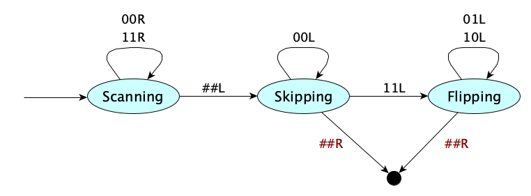
Another example: the multiply-by-four machine that we’ve seen before:

has this compact table (since we are not using No-moves, I swapped that N or an R):

	0	1	#
A	0RA	1RA	0RB
B	—	—	0RC
C	—	—	—

And for the binary increment machine,

we have:

	0	1	#
A	0RA	1RA	#LB
B	1LC	0LB	1LC
C	—	—	—

Annoyances!

The last move before entering the final state is so...arbitrary! It is a downside of the standard format.

Not sure if it is worth complaining about.

To paraphrase Stroustrup: there are two kinds of computation models, those that people complain about and those that no one uses.

The Halting Pseudo-State Variety

A slightly different definition of a deterministic Turing Machine treats “halting” as a kind of state, a halting pseudo-state:

$$ \delta : (Q \times \Gamma) \rightarrow \Gamma \times \{\textsf{L}, \textsf{R}\} \times (Q\cup \{ \textsf{HALT} \}) $$

This says: if the machine is in some state $\sigma \in Q$, and currently looking at a symbol $\sigma \in \Gamma$, then:

1. Replace the symbol with a new symbol $\sigma'$, move one cell, THEN
2. Either enter state $q' \in Q$ or Halt

For this variety, the special halting pseudo-state has no outgoing transitions. It is never listed in the left column (as you can tell from the type of the transition function). Sometimes, it’s like we have fewer “real” states. So, for example, in the increment machine, we replace the old Incremented state with a halting pseudo-state:

We get the following table, where the halt state shows up as a Z (or an H, or any other character that does not name a regular state):

	0	1	#
A	0RA	1RA	#LB
B	1LZ	0LB	1LZ

Here’s the multiply-by-four machine, withe the old Quadrupled state now a halt pseudo-state. We had to add in some new explicit transitions (because determinism can be clunky):

	0	1	#
A	0RA	1RA	0RB
B	0RZ	0RZ	0RZ

For negation, the existing machine did not have a “natural” halting state, so we have to add one explicitly (again, with silly arbitrary moves before entering the halt state...ugh):

	0	1	#
A	0RA	1RA	#LB
B	0LB	1LC	#RZ
C	1LC	0LC	#RZ

On the Number of Possible Deterministic TMs

How many $n$-state deterministic TMs are there?

For a tape alphabet of $k$ symbols, it turns out that for the halt-as-action variety, there are $(2kn+1)^{kn}$ machines, and for the halt-as-state variety, there are $(2k(n+1))^{kn}$ machines.

For the $k=2$ case, the numbers are $(4n+1)^{2n}$ and $(4(n+1))^{2n}$, respectively.

We will work this out. It is good to practice our discrete math skills when learning computing theory.

Does determinism reduce the power of a TM?

A fun fact: Changing the model of TMs from “in configuration $(q,\sigma)$ choose any one of the following action-move operations” (nondeterministic) to “in configuration $(q,\sigma)$ do this exact action-move” (deterministic) does not change the computing power of the model. Anything computed by a deterministic TM can be computed by a regular TM and vice versa. This may or may not be obvious to you.

Does determinism reduce the power of a restricted TM?

Glad you asked:

• For FAs, no!
• For PDAs, yes!
• For LBAs, unknown!

Online Simulators

When writing a Turing machine to carry out a computation or decide a question, don’t just guess! There are a couple of online simulators out there, such as this one and this one and this one so you can check your work! Not surprisingly, they all employ different variations in the way machines are representing, but they’re all computationally equivalent.

Recall Practice

Here are some questions useful for your spaced repetition learning. Many of the answers are not found on this page. Some will have popped up in lecture. Others will require you to do your own research.

1. What were the three main approaches to mathematical foundations in the late 19th and early 20th century?
   Formalism, Logicism, Intuitionism
2. What is formalism?
   The view that mathematics is just a game played with symbols according to rules.
3. What is logicism?
   The view that mathematics can be reduced to logic.
4. What is intuitionism?
   The view that mathematics is a mental construct, and that only constructive proofs are valid.
5. What was the Entscheidungsproblem?
   The challenge to find a mechanical procedure to determine whether a mathematical statement was provable from its axioms.
6. What was necessary to show that Entscheidungsproblem had no solution?
   A precise definition of computation.
7. Who were the main players in defining computation and what were their approaches?
   Gödel (logical), Church (lambda calculus), Turing (mechanistic).
8. How did Turing come up with the idea of a Turing machine?
   By abstracting the essential features of computation, gleaned from observing the (human) computers of his day.
9. What were some of the simplifications Turing made in his machine model?
   (1) Instead of a 2-D sheet of paper, a single tape, and (2) a read-write head that moves one cell at a time.
10. What are the four columns of a Turing machine instruction table, as Turing originally defined them?
    Current State, Current Symbol, Actions (Write/Move), Next State
11. How are the transitions labeled in a Turing machine diagram?
    current-symbol / comma-separated actions. Actions are either a symbol to write or a move direction (L or R).
12. A simplified TM table has five columns. What are they?
    Current State, Current Symbol, Write Symbol, Move Direction, Next State
13. How is the input of a Turing machine represented?
    As a string of symbols on the tape, with the rest of the tape blank.
14. What is the output of a (transducer) Turing Machine?
    The contents of the tape when the machine halts, between the infinite runs of blanks.
15. How is a recognizer Turing Machine’s output represented?
    If the machine halts in an accept state, the answer is YES; if it halts in a non-accept state, the answer is NO; if it never halts, no answer is given.
16. How does a TM to determine whether a binary number is even work?
    It scans to the end of the input and checks whether the last symbol is 0, and if it is, enters an accept state and halts. If there is no last symbol or the last symbol is a 1, it halts in a non-accept state.
17. How does a TM to determine whether a binary number is negative work?
    It checks the first symbol and accepts if it is a 1.
18. In the formal definition of a TM, what are the two alphabets $\Sigma$ and $\Gamma$?
    $\Sigma$ is the input alphabet, and $\Gamma$ is the tape alphabet, which includes $\Sigma$ and the blank symbol.
19. What do recognizing TMs have in their formal definition that transducer TMs do not?
    A set of accept states $A$.
20. What is the difference between a recognizer and a decider?
    A decider always halts with a YES or NO answer, while a recognizer may loop forever on some inputs.
21. How can TMs be encoded as strings?
    By concatenating the transition table rows in a compact format.
22. Given a Turing Machine $M$, how do we denote its encoding?
    $\langle M \rangle$
23. What is a Universal Turing Machine?
    A TM that can simulate any other TM given its encoding and input.
24. How is the Universal Turing Machine formally defined?
    $U(\langle M \rangle\texttt{#}x) = M(x)$
25. What is the significance of the Universal Turing Machine?
    It shows that a single machine can perform any computation that any TM can, laying the foundation for general-purpose computers.
26. What are common variations to a TM regarding moves?
    (1) After reading and possibly writing, don’t move at all, (2) Move without reading.
27. What are some common variations to the tape structure of a TM?
    (1) One-way infinite tape, (2) Multi-dimensional tape, (3) Multiple tapes, (4) Stack-like or Queue-like tapes, (5) Read-only or write-only tapes, (6) Bounded tapes.
28. Which of the following modifications to the TM actually reduce its computing power? (a) one-way infinite tape, (b) multi-dimensional tape, (c) multiple tapes, (d) single-stack-like tape, (e) double-stack-like tape, (f) queue-like tape, (g) tape bounded at both ends.
    Only (d) single-stack-like tape and (g) tape bounded at both ends reduce computing power.
29. What are the three best-known restricted forms of TMs that actually reduce computing power?
    (1) Linear Bounded Automata (LBAs), (2) Pushdown Automata (PDAs), (3) Finite Automata (FAs).
30. What is an LBA?
    A Turing Machine with a tape of a fixed bounded length, and a transition function that can take into account what to do when at the tape boundaries.
31. What is a PDA?
    A Turing Machine with a stack-based working memory separate from its read-only input tape, and in which the input is read from left-to-right with no way to go backwards.
32. What is an FA?
    A Turing Machine with a finite tape consisting only of the input, and that reads the input from left to right without the ability to write or move backwards.
33. What is a deterministic Turing Machine?
    A TM where for every state and symbol, there is exactly one possible transition.
34. What are the two common ways to represent halting in a deterministic TM?
    (1) a special halt action (lack of a transition for the current state and symbol) or (2) as a special halt pseudo-state.
35. What is the type of the transition function for the halt-as-action deterministic Turing Machine?
    $$ \delta : (Q \times \Gamma) \rightarrow (\Gamma \times \{L, R\} \times Q) \cup \{ \textsf{HALT} \} $$
36. What is the type of the transition function for the halt-as-pseudo-state deterministic Turing Machine?
    $$ \delta : (Q \times \Gamma) \rightarrow \Gamma \times \{L, R\} \times (Q\cup \{ \textsf{HALT}\}) $$
37. Do deterministic TMs have the same computing power as non-deterministic TMs?
    Yes.
38. Do deterministic PDAs have the same computing power as non-deterministic PDAs?
    No.
39. Do deterministic FAs have the same computing power as non-deterministic FAs?
    Yes.
40. Do deterministic LBAs have the same computing power as non-deterministic LBAs?
    We don’t know yet.

Summary