Automata Theory
Motivation
The field we now call automata theory arose from many different areas of research, including:
- Mathematics, through attempts to formalize the meaning of computation
- Engineering, through attempts to characterize (discrete) physical systems
- Psychology, through attempts to characterize human thinking and reasoning
These folks all came up with the notion of an automaton as a kind of machine, real or abstract, that runs by itself (hence the prefix “auto”) to process some information. There should be no limits to your imagination regarding how an automaton should or should not look, nor what kinds of internal operations it carries out (as long as it is finitely describable).
A brief history of the field can be found at Wikipedia.
We want a rigorous theory of automata. Therefore, we will make the following assumptions about the automata that we study:
- A machine must have a finite description.
- The input to the machine is represented as finite string of symbols from a finite alphabet.
- Each computational “step” must take a finite amount of time.
The first assumption is reasonable because a machine that requires an infinite description could not be built, let alone understood. The second assumption is reasonable for reasons we discussed previously in our notes on language theory.
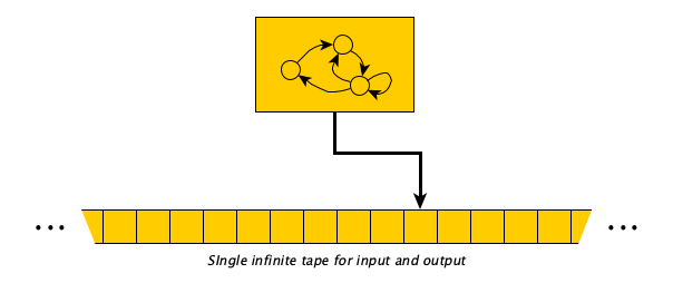
We can give a picture of an automaton as follows:
For computations with multiple inputs, we can make a single string with a special separator symbol.
Why create and study a theory of automata? Two reasons:
- It gives us a framework in which we can ask what computation is, what we can compute, what is necessary (e.g. time and space) for computation, and how computations can be carried out.
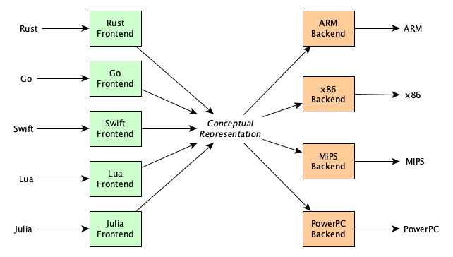
- It provides insights into how we can design and build both real and abstract machines—and even programming languages! Abstract machines are quite important because they show how to carry out computations independent of any real machine and independent of any real high-level programming language, allowing us build multi-language compiler systems (where the abstract machine serves as a conceptual representation of a program):
Plan of Study
Here’s how we’ll proceed:
- We’ll look at actual computational models, or automata, that people have created.
- We’ll make some useful generalizations, classifying automata across several dimensions.
- We’ll look at how automata theory is related to language theory, computability theory, and complexity theory.
- We’ll look at applications, specially how various virtual machines have grown out of the theory.
Classic Examples of Automata
We will look at examples first, because knowledge advances by people make things before they generalize what they have done into theories.
Turing Machines (TMs)
Turing Machines are so historically significant and influential, that I have an entire separate page of notes for them, including how Turing came up with the idea and design. For now, let’s just look at the basics.
In a TM, we begin with the input sitting on an infinite tape of cells surrounded by blanks. The machine has a head pointing to the first symbol of the input. The machine’s control is a finite set of rules that says “If in state $q$ looking at symbol $\sigma$, then (1) optionally replace the current symbol with a different symbol $\sigma'$, (2) optionally move either one cell right or left, and then (3) optionally transition to a different state $q'$.” The machine computes by following the rules one after the other. When it gets to a configuration in which there is no rule for the current state and currently scanned symbol, it halts.
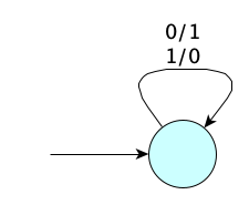
We’ll cover Turing Machines in detail later, but for now here’s an example Turing Machine to increment a binary number:
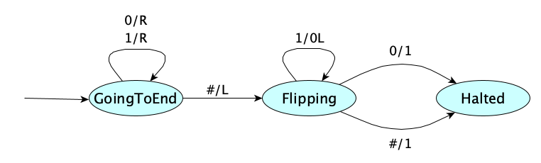
Here is the machine in action, incrementing 100111:
            S
──┬───┬───┬───┬───┬───┬───┬───┬───┬───┬──
  │ # │ # | 1 | 0 | 1 | 1 | 1 | # | # |
──┴───┴───┴───┴───┴───┴───┴───┴───┴───┴──

                S
──┬───┬───┬───┬───┬───┬───┬───┬───┬───┬──
  │ # │ # | 1 | 0 | 1 | 1 | 1 | # | # |
──┴───┴───┴───┴───┴───┴───┴───┴───┴───┴──

                    S
──┬───┬───┬───┬───┬───┬───┬───┬───┬───┬──
  │ # │ # | 1 | 0 | 1 | 1 | 1 | # | # |
──┴───┴───┴───┴───┴───┴───┴───┴───┴───┴──

                        S
──┬───┬───┬───┬───┬───┬───┬───┬───┬───┬──
  │ # │ # | 1 | 0 | 1 | 1 | 1 | # | # |
──┴───┴───┴───┴───┴───┴───┴───┴───┴───┴──

                            S
──┬───┬───┬───┬───┬───┬───┬───┬───┬───┬──
  │ # │ # | 1 | 0 | 1 | 1 | 1 | # | # |
──┴───┴───┴───┴───┴───┴───┴───┴───┴───┴──

                                S
──┬───┬───┬───┬───┬───┬───┬───┬───┬───┬──
  │ # │ # | 1 | 0 | 1 | 1 | 1 | # | # |
──┴───┴───┴───┴───┴───┴───┴───┴───┴───┴──

                            F
──┬───┬───┬───┬───┬───┬───┬───┬───┬───┬──
  │ # │ # | 1 | 0 | 1 | 1 | 1 | # | # |
──┴───┴───┴───┴───┴───┴───┴───┴───┴───┴──

                        F
──┬───┬───┬───┬───┬───┬───┬───┬───┬───┬──
  │ # │ # | 1 | 0 | 1 | 1 | 0 | # | # |
──┴───┴───┴───┴───┴───┴───┴───┴───┴───┴──

                    F
──┬───┬───┬───┬───┬───┬───┬───┬───┬───┬──
  │ # │ # | 1 | 0 | 1 | 0 | 0 | # | # |
──┴───┴───┴───┴───┴───┴───┴───┴───┴───┴──

                F
──┬───┬───┬───┬───┬───┬───┬───┬───┬───┬──
  │ # │ # | 1 | 0 | 0 | 0 | 0 | # | # |
──┴───┴───┴───┴───┴───┴───┴───┴───┴───┴──

                I
──┬───┬───┬───┬───┬───┬───┬───┬───┬───┬──
  │ # │ # | 1 | 1 | 0 | 0 | 0 | # | # |
──┴───┴───┴───┴───┴───┴───┴───┴───┴───┴──
A variation on the Turing Machine is to make each action be comprised of a mandatory print and a mandatory move. In that variation, the state diagram for our binary number increment machine would be written like so:

The mandatory move part is a little annoying, since there is often a useless move at the end of a computation (as in the above example). If it is too annoying, then add to L and R the value N, for “no move” or “neutral”.
Get used to multiple variations and notationsIt turns out there are way more than two variations of the Turing Machine, and the notations can vary quite a bit. They all have in common that “when in state $q$ looking at $\sigma$, optionally perform actions then optionally transition to a new state”.
These notes will use both transition notations (e.g.,
0→Rfor zero-or-more actions at a time and00Rfor exactly-one-write-and-one-move), so get used to reading both. They are equivalent in computing power.
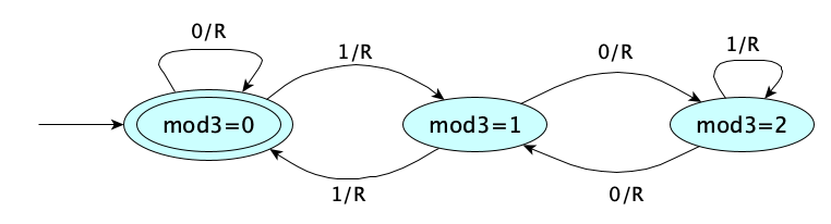
Generally, when the machine halts, the result of the computation is whatever is left on the tape (between the infinite runs of blanks). But sometimes, we want a computation that just answers a YES-NO question. In these cases, it is super super convenient to not have to actually write YES or NO, but instead introduce the notion of an accept state. Stopping in an accept state means the answer is YES. Such a machine is called a recognizer because it just recognizes which inputs produce a YES answer. A machine intended to produce actual output data is called a transducer. Here is a recognizer to determine if its input, a binary number, is divisible by three:
Jade has a little explainer on Turing Machines (in which she uses the notation for the exactly-one-print, exactly-one-move model):
Watching videos can be super helpful, but you’ll want to follow up with practice.
Pretend you are Turing machine. Painstakingly work out the computations of incrementing the binary number 11010011111, and determining whether 11010011111 is divisible by three. Write out each “configuration” (state and tape contents) you pass through.
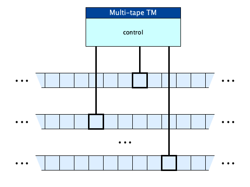
Multi-tape Turing Machines
We’ll see later that this “single-tape” Turing Machine is, as far as we know, capable to computing all computable functions. It’s simplicity makes it the go-to model for studying computation! But for convenience, we can extend the model with multiple tapes! This doesn’t add any more computing power: you can show that any TM with multiple tapes can be simulated with a 1-tape TM.
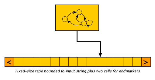
Linear Bounded Automata (LBAs)
Single and multi-tape Turing Machines have equal computing power. Thanks to their infinite tapes, they have a lot of power. What if we bound the tape?
A Linear Bounded Automaton, or LBA, is essentially a Turing Machine whose tape is not infinite but rather is bounded to the size of its input plus two additional read-only cells: one to the left of the input containing an non-replaceable “left-end-marker symbol” and one to the right containing a non-replaceable “right-end-marker” symbol. The machine is not allowed to move beyond these markers, nor is it allowed to write the marker characters anywhere else on the tape. It may, of course, freely write any non-marker symbol between the markers.
It feels a little more realistic, closer to a real computer, because of it having a finite “memory,” right?
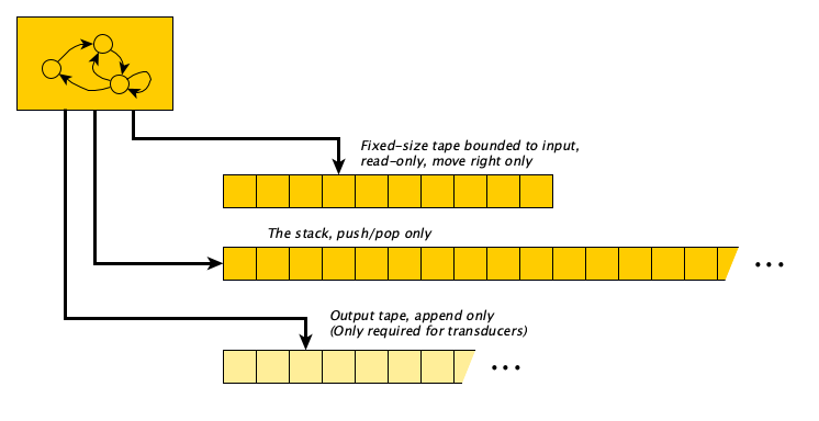
Pushdown Automata (PDAs)
Turing Machines and LBAs can move back and forth across their tapes. There’s an interesting restriction you can make that requires you to read through the input exactly once from left to right only, and only use a stack for working memory. Why might this be nice? Stack push and pop, you may remember, are $\Theta(1)$ (constant) time operations.
A Pushdown Automaton, or PDA, is essentially a Turing Machine with (1) a read-only input tape with no left moves allowed, (2) a separate unbounded stack that is initially empty, and (3) optionally, an append-only output tape. The transition rules always take into account the current state, but may also consider the current input symbol (in which case the input head is advanced to the right) and may also consider the symbol on the top of the stack (in which case it is popped). The action fired by a rule is to (optionally) push symbols on the stack, (optionally, if a transducer) append symbols to the output tape, and (optionally) move to a new state.
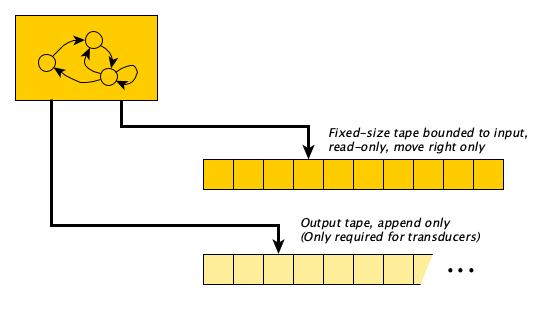
Finite Automata (FAs)
Some problems don’t need any memory at all. Just zoom through the input one symbol at a time and be done!
A Finite Automaton or FA, is a Turing Machine with a read-only input tape and a head that moves one cell to the right at every step (there are no left-moves and no no-moves). Optionally, it may produce output on a separate write-only tape that is initially blank and only appended to.
It’s FA, not FSMSometimes you will hear folks call an FA a “finite state machine” or FSM for short. This is confusing because all automata have a finite number of states. Also, the acronym FSM is easily confused with the deity of Pastafarianism.
When describing FAs, we don’t have to worry about blanks, or say whether we are moving left or right! All we need is the input symbol and the output symbol(s). For a first example, here is a transducer FA that computes the one’s complement of its input:
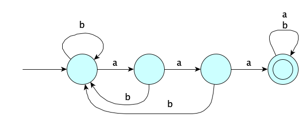
For recognizers, we don’t have any output at all, so the machine transitions just have the input symbol. Here’s an FA to determine whether its input has three consecutive $a$’s somewhere:
An FA that writes to its output on a transition is called a Mealy Machine. You can also make an FA transducer that outputs a symbol whenever it enters a state; this would be called a Moore Machine.
Queue Automata
A queue automaton is a TM that, instead of moving left or right at each step, instead always dequeues the symbol at the left and enqueues some other string of symbols on the right.
Rewrite Machines
We can mechanically compute by applying rules (from a finite set of rules) that allow us to rewrite part of a string into another. We start with the input surrounded by begin and end markers [ and ], and keep rewriting until there are no more rules to apply.
For example, here’s an instruction set for a rewrite machine that increments binary numbers:
Some example runs:
- $[0] \Longrightarrow [Y1 \Longrightarrow 1$
- $[1] \Longrightarrow [X0 \Longrightarrow 10$
- $[101] \Longrightarrow [10X0 \Longrightarrow [1Y10 \Longrightarrow [Y110 \Longrightarrow 110$
- $[110010] \Longrightarrow [11001Y1 \Longrightarrow [1100Y11 \Longrightarrow [110Y011 \Longrightarrow \cdots \Longrightarrow [Y110011 \Longrightarrow 110011$
- $[111] \Longrightarrow [11X0 \Longrightarrow [1X00 \Longrightarrow [X000 \Longrightarrow 1000$
- $[\,]$ cannot be reduced, it’s an illegal input with an illegal output
How about a formal definition?
A rewrite machine is a tuple $(\Sigma, R)$ where:
- $\Sigma$ is the alphabet of symbols
- $R \subseteq \Sigma^* \times \Sigma^*$ is the rewriting relation.
The one-step derivation relation $\Longrightarrow_R \;\subseteq \Sigma^* \times \Sigma^*$ is defined as: $xuy \Longrightarrow_R xvy$ iff $u R v$.
A rewrite machine $(\Sigma, R)$ computes output $w'$ from input $w$ iff $$[w] \Longrightarrow^*_R w' \wedge \forall\,x\,y\,z . w' = xyz \supset \neg \exists u . yRu$$
We can make a rewrite machine be a recognizer, too. Here is a rewrite machine that determines whether or not its input is in the form $a^nb^nc^n$, for $n \geq 0$:
That might have been simpler than you thought it might be, given the complexity of the analytic grammar, the generative grammar, and even the Turing Machine we saw for this language earlier!
Let’s extend the definition above:
A rewrite machine $(\Sigma, R)$ accepts $w$ iff $[w] \Longrightarrow^*_R \fbox{YES}$
Register Machines
Now let’s make something a bit less primitive and way more useful.
A register machine has a number of registers $r_0, r_1, r_2, \ldots$, each holding a single (unbounded) natural number. The machine’s control is a program, defined as a list of (labeled) instructions. The instructions are normally executed in sequence, but some instructions can cause a “jump” to an arbitrary instruction. The instruction set varies from model to model (of which there exist an infinite number of possibilities). Here’s an example of a register machine with a very small instruction set:
| Instruction | Description |
|---|---|
| $\textsf{load } r_k, n$ | $r_k := n$ |
| $\textsf{copy }r_i, r_j$ | copy contents of $r_j$ into $r_i$ |
| $\textsf{add } r_i, r_j, r_k$ | Store sum of contents of $r_j$ and $r_k$ into $r_i$ |
| ... and so on for $\textsf{sub}$, $\textsf{mul}$, $\textsf{div}$, $\textsf{pow}$, $\textsf{and}$, $\textsf{or}$, $\textsf{lt}$, $\textsf{le}$, $\textsf{eq}$, $\textsf{ne}$, $\textsf{ge}$, $\textsf{gt}$, $\textsf{shl}$, $\textsf{shr}$ | |
| $\textsf{neg } r_i, r_j$ | Store negation of the contents of $r_j$ into $r_i$ |
| $\textsf{not } r_i, r_j$ | Store bitwise negation of the contents of $r_j$ into $r_i$ |
| $\textsf{jump } n$ | Jump ahead (or back, if $n$ is negative) $n$ instructions |
| $\textsf{jz } r_i, n$ | Jump ahead (or back, if $n$ is negative) $n$ instructions if contents of $r_i$ is $0$ |
Register machines are rather important, as they are pretty much the basis for most “real” machines today. We’ll discuss them in more detail later, where we will connect them with modern machines with large and powerful instruction sets.
Stack Machines
A stack machine is pretty much a register machine where the register operands are implicit: the register sequence is treated as a stack. We’ll see them in details in the notes on register machines.
They are very popular because of their simplicity. In fact, the operation of the JVM and WebAssembly is based on stack machines.
And More!
Yes, people have created probabilistic automata and quantum automata, too.
Not to mention Büchi, Rabin, Strett, Parity, Muller, Analog, Continuous, and Cellular automata. There are no doubt others.
Oh, and do check out the amazing SECD Machine, designed to evaluate lambda calculus expressions. It’s a bid of hybrid, containing components from different models.
Classifying Automata
Now that we’ve seen specific automata, we can now generalize and come up with a useful vocabulary.
There are many dimensions on which we can characterize automata:
- (Control) How does the machine represent and execute each step of a computation?
- (Memory) Where are the inputs, outputs, and scratch data stored?
- (Output) Is the machine just answering a YES/NO question or computing a result?
- (Architecture) Is the program hard-wired into the machine, or stored in memory with data?
- (Synchronization) Synchronous vs. asynchronous
- (Execution) Sequential vs. parallel
- (Determinism) Deterministic vs. non-deterministic
- (Tolerance) Definite vs. probabilistic
- (Information) Classical vs. quantum
- (Pragmatic) Minimal as possible (theoretically valuable, but hard to work with in practice) vs. complex (easier for humans to work with)
But as these notes are introductory, we will focus only on the first four dimensions.
Control Variations
There are different ways to specify the operation of an automaton. The main options are (1) state machines, (2) instruction sets, and (3) rewrite rules.
- A state machine automaton performs a computation by moving through states that indicate in which phase of the computation one is in. The “program” is basically a transition table. The computation ends when you land in a state that doesn’t have a transition out of the current state for the current machine configuration. Transition tables come in many forms, depending on the type of state machine, but are generally structured like so:
If you are in
this stateand this
event occursThen perform
this actionand move
to stateState machines can also be given with pictures:
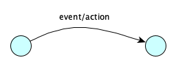
If there can be more than one action/transition to take from a given state/input configuration, the machine is said to be non-deterministic, otherwise it is deterministic.
- An instruction-set machine has a control made up of a list of instructions. Typically, instructions are executed in order, but some machine operands can be references to other instructions (e.g., via labels or by position) to allow conditional and iterative execution. Instructions that directly reference other instructions to explicity change the control flow are called branches or jumps.
┌───────────────────┐
│   Instruction 0   │
├───────────────────┤
│   Instruction 1   │
├───────────────────┤
│   Instruction 2   │
├───────────────────┤
│         .         │
│         .         │
│         .         │
├───────────────────┤
│  Instruction n-1  │
└───────────────────┘
Register machines are by nature deterministic, but you can fake nondeterministic behavior by introducing an instruction that randomly chooses between multiple next instructions.
- A rewrite machine is an automaton specified with a set of rewrite rules that successively replace substrings of an input string until it is transformed into the output. The “program” defined by a rewrite system is something like:
Rewrite machines are inherently nondeterministic, though if you were force computation to proceed by always choosing the first applicable rule in some fixed order (say, always the leftmost or always the rightmost), your computation would be deterministic.If you see this substring Rewrite with this substring
The three operational variations are convenient, but neither is really any more computationally powerful than the other. Each can simulate the others.
Memory Variations
There’s a lot of variety in memory, but two primary kinds are:
- Tapes: a tape is sequence of cells, each holding a single symbol. At a given point in time, the machine is looking at a current cell on the tape. The machine “moves” left or right during computation. The tape can have a finite number of cells, or can be infinite in one direction, or infinite in both directions. A machine can have multiple tapes. There are models where tapes are restricted to be read-only, write-only, stack-like (push/pop only), or queue-like (enqueue/dequeue only).
─┬───┬───┬───┬───┬───┬───┬───┬───┬───┬─ • • • │ │ | | | | | | | | • • • ─┴───┴───┴───┴───┴───┴───┴───┴───┴───┴─ - Registers: A machine can have one or more registers. Each register holds some data. Usually in automata theory, a register holds a natural number (nonnegative integer) of unbounded size, but variations allow it to hold only a single symbol, or maybe a floating-point (but not real) number, or even a string. Registers are numbered $r_0, r_1, r_2, \ldots$ and they can be accessed by their number. Some models have a finite number of registers; in others, infinite. There can even be different classes of registers: for example, maybe only certain registers can do arithmetic, maybe only certain registers can be used for indirect addressing, etc.
       ┌────────────────────┐
    r0 │                    │
       ├────────────────────┤
    r1 │                    │
       ├────────────────────┤
    r2 │                    │
       ├────────────────────┤
    r3 │                    │
       ├────────────────────┤
    r4 │                    │
       ├────────────────────┤
What other kinds of memory can you come up with?
One idea: multi-dimensional tapes, which would allow for, say, up, down, left, and right movements, and perhaps more. Use your imagination to build new computing machines.
Output Variations
Here’s an unnecessary distinction, but one that is super convenient to make.
- A transducer automaton transforms an input into an output (if it finishes):
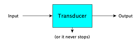
- A recognizer automaton accepts or rejects its input, by answering a YES-NO question about the input (if it finishes):
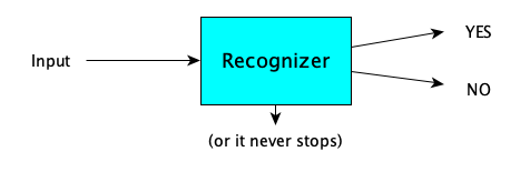
If a recognizer machine $M$ says YES to input $w$, we say that $M$ accepts $w$.
A recognizer that always finishes and answers YES or NO (and never loops) is called a decider.
Architectural Variations
One final variation of interest, applicable to instruction-based automata only, really, is: where are the instructions stored? There are two main architectures:
- Harvard Architecture: Instructions are stored in a dedicated, read-only instruction unit, separate from data.
- Von Neumann Architecture: Instructions are stored together with the data.
Review
Here’s a table summarizing the variations we’ve discussed:
| Dimension | Options | Description |
|---|---|---|
| Control | State machine | Control is a states with transitions |
| Instruction list | Control is a list of instructions (which may contain jumps) | |
| Rewrite rules | Rules successive rewrite portions of the data | |
| Memory | Tapes | Located by moving through the cells one at a time |
| Registers | Located by register index | |
| Output | Transducer | Produces an arbitrary output |
| Recognizer | Outputs YES or NO only | |
| Architecture | Harvard | Code is separate from the data |
| Von Neumann | Code and data are stored together |
Connections To Formal Languages
A recognizer automata actually defines a formal language! That is, the language of recognizer machine $M$, or the language recognized by $M$, is:
$$ L(M) = \{ w \mid M \textrm{ accepts } w \} $$Nice! This means a formal language can be defined by not only by a grammar but also by a machine. This is philosophically interesting, if not profound.
The notions of “decision problem” and “language” are interchangeable.
Also if $L$ is a language, then $M_L$ is a recognizer machine for $L$.
How about an example, to understand the important concepts here, and to get the vocabulary right? Let $M$ be the Turing Machine given by the following state diagram:
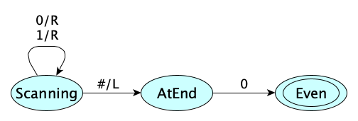
When run on any non-blank input of binary digits, the machine will end in the accept state iff the input ends with a 0. Otherwise it will get stuck. Therefore we say:
- $M$ accepts the string $110100100$
- $M$ recognizes the language $\{ w \in \{0,1\}^* \mid w \textrm{ is an even binary integer} \}$
- $M$ accepts the language $\{ w \in \{0,1\}^* \mid w \textrm{ is an even binary integer} \}$
- $M$ decides the language $\{ w \in \{0,1\}^* \mid w \textrm{ is an even binary integer} \}$
- $L(M) = \{ w \in \{0,1\}^* \mid w \textrm{ is an even binary integer} \}$
- If we define $EVEN$ as $ \{ w \in \{0,1\}^* \mid w \textrm{ is an even binary integer} \}$ then $M_{EVEN} = M$
Accepting vs. DecidingIn tne example above, the machine $M$ did indeed both accept and decide the language of even binary integers. However, there do exist languages that are recognizable by a TM but not decidable by any TM. The line between the acceptable and the decidable is part of computability theory, which we’ll study later.
It turns out that different kinds of (recognizer) machines can recognize different classes of languages. Here is a progression of machine types with strictly increasing recognition power:
| Automata | Languages that can recognized |
|---|---|
| Loop-free FA | Finite Languages (languages with a finite number of strings). |
| FA | Regular Languages. You can recognize these without any external memory whatsoever. The only “memory” (if you can call it that) is where we are in the input and what state we are in. These languages are recognizable in linear time. |
| Deterministic PDA (DPDA) | Deterministic Context-Free Languages. An interesting subset of the context-free languages that show up in parsing theory. |
| Nondeterministic PDA (NPDA) | Context-Free Languages. Recognized by only using stack memory, which is super fast. |
| LBA | Type-1 Languages. Who knew? Bounding the tape of a TM reduces the computing power significantly! |
| TM that always halts | Decidable Languages. Also known as the Recursive Languages, $R$. |
| TM | Type-0 Languages. Recursively Enumerable Languages, $RE$. For languages that are in $RE$ but not in $R$, a TM can be found that will accept (say YES) every string in the language, but will not be able to halt and say NO for all strings not in the language. |
DeterminismMachines that allow more than one possible operation from a given configuration are called nondeterministic, and those that allow only one are called deterministic. Okay, fine, but here’s the philosophical question: is nondeterminism more “powerful” than determinism? That is, can we recognize more languages with nondeterministic machines of a given class than deterministic ones? It turns out:
- For FAs and TMs, there is NO difference in recognition power between deterministic and nondeterministic versions.
- For PDAs, there IS a difference in recognition power between deterministic and nondeterministic versions.
- For LBAs, we don’t know!
Who knew right? 🤯
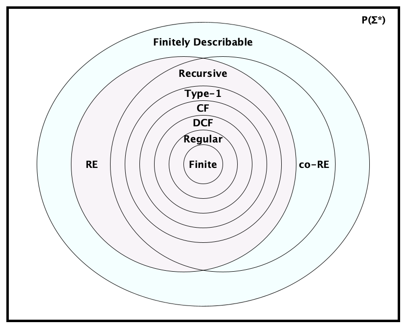
These classes form a hierarchy of language recognition power, with each language class being a proper subset of the next. Here’s another view of the table above, illustrating the containment relationships, with example languages in each region:
There were new languages there!You may have noticed the languages $PRESBURGER$, $H$ and $\overline{H}$ in the diagram above. We haven’t seen them yet. But we will. For now, just note that it is pretty cool that we can identify languages in some of these interesting families.
In many cases, the class of languages accepted by a type of particular machine correspond exactly to the class of languages generated by a type of grammar. And for those language classes that cannot be characterized by a grammar, there are no automata that characterize them either!
| Language Type | Description | Grammar | Recognizer |
|---|---|---|---|
| Finite | A language with only a finite number of strings. | $S \rightarrow w_1 | \ldots | w_n$ | Loop-free FA |
| Regular (Type 3) |
A language in which strings can be recognized by processing them one symbol at a time, without backtracking, and without using additional memory. | RLG LLG |
FA |
| Deterministic Context Free (LR) |
A language recognizable on a deterministic PDA. (Stacks are nice! Θ(1) access! Determinism is nice too! Much more efficient.) | LR | DPDA |
| Context Free (Type 2) |
A language recognizable on a nondeterministic PDA. (Stacks are nice! Θ(1) access! But with nondeterminism, recognition is slower.) | CFG | PDA |
| Context Sensitive (Type 1) |
A language recognizable on an LBA. (The name “context-sensitive” is confusing because intuitively all languages “beyond” Type 1 in the hierarchy are sensitive to context). | ENCG CSG |
LBA |
| Recursive (R) | A language in which string membership is decidable. There are no predetermined memory bounds, and no bounds on the number of steps. | (No name) | TM that always halts |
| Recursively Enumerable (Type 0 / RE) |
A language in which string membership is partially decidable: if a string is in the language, you can determine that for sure; if a string is not, you might not be able to determine this. | Grammar | TM |
| co-RE | A language whose complement is RE. If a string is not in the language, you can determine that for sure; if a string is in the language, you might not be able to determine this. | Not computable | |
| Finitely Describable | A language that has a finite description | Not computable | |
| All Languages ($\mathcal{P}(\Sigma^*)$) |
All possible languages over the alphabet | Not computable | |
Fun fact: $\textit{RE} \cap \textit{co-}RE = R$.
The language class RE lines up with what we understand to be computable.
Connections To Computability Theory
Can any type of automata, or other computational model, compute a larger class of functions than a Turing Machine? We don’t think so. In fact, the following are all equal in computing power:
- Turing Machines
- Deterministic TMs
- One-way infinite tape TMs
- Multi-tape TMs
- Multi-dimensional TMs (e.g., can move N, E, S, W)
- Queue Automata
- NPDAs with two stacks
- Register Machines
- RAMs
- RASPs
- The μ-recursive functions
- Post Systems
- Phrase-Structure (Type-0) Grammars
- The Lambda Calculus
The fact that these all are essentially the same thing, and all attempts at making them more powerful don’t actually increase their power, led to the Church-Turing Thesis, which states:
The Turing Machine captures exactly we intuitively think of as computable.
Connections to Complexity Theory
There are hundreds (no kidding) of other classes of languages. Perhaps the two most famous are:
- $\mathit{P}$: The set of all languages that can be recognized by a deterministic TM in a number of steps bounded by a fixed polynomial in the size of the input.
- $\mathit{NP}$: The set of all languages that can be recognized by a TM in a number of steps bounded by a fixed polynomial in the size of the input.
Note, by definition, $\mathit{P} \subseteq \mathit{NP}$, but no one has been able to prove whether or not $\mathit{P} = \mathit{NP}$. There is a cash prize waiting for you if you can do it.
The language classes discovered and invented in the study of complexity theory can be mixed into the language classes we’ve seen already. Gabe Robins created this beautiful visualization:
There’s so much more, including languages tied to probabilistic and quantum computing. All of the language families described above, as well as hundreds more, can be found in the Complexity Zoo.
Applications
One of the reasons we have theories is to apply them. (Remember, a theory is an organized body of knowledge with explanatory and predictive powers.) What are some applications of automata?
Language Processing
Type-3 machines are used in Lexical Analysis, (extracting “words” from a string of characters), an important operation in text processing, and especially in compiler writing.
Type-2 machines are used in Parsing, uncovering the structure of a string of symbols, another hugely important and common operation.
Instruction-Oriented Languages
Automata Theory, like any theory, has its small building blocks. We aim for machines that are so small and so easy to understand, that their operation can be fully grasped and analyzed. If the operations are instructions, and we have a way to represent these instructions, we have an interesting blurring between instructions and machines.
Brainfuck
Brainfuck (or Brainf**k as it is commonly known) is a programming language with an explicit machine execution model featuring (1) a fixed program stored on a read-only tape where each cell holds one of eight instructions, (2) a read-only input stream of bytes (you can think of it as a tape), (3) a write-only output stream of bytes (also a tape), and (4) a data tape with a fixed left end and infinite to the right (although really the language specification says at least 30,000 cells). The eight instructions are:
| Instruction | Description |
|---|---|
+ | Increment the byte in the current data cell |
- | Decrement the byte in the current data cell |
. | Output the byte in the current data cell |
, | Read next byte from input and store in current data cell |
< | Move left on tape |
> | Move right on tape |
[ | If byte in current data cell is 0, jump to instruction right after the next matching ] |
] | If byte in current data cell is not 0, jump to instruction right after the previous matching [ |
Here’s a program in the language. Can you figure out what it does?
+++++++[>+++++[>++>+++<<-]<-]>>++.>.
Need a hint?
7  5   2    3
7  0  10   15
0  0  70  105
      72  105
See the Language overview at Esolang, the Wikipedia article, and this collection of example programs.
$\mathcal{P''}$
$\mathcal{P''}$ is one of the earliest of the tiny languages. Its alphabet is only four symbols, each mapping to a specific instruction. It’s perhaps too small to easily study, but fascinating for its minimalism.
Stack-Based Languages
We’ll cover some of these in class.
Turing Machines as a Programming Language
Think about it: when you give the encoding of a Turing machine, aren’t you in some sense expressing a computation? Machine descriptions are communicated in a language, so they can be viewed as a program. We’ll provide only a simple example, which will be “run” in class:
SCANNING,0,0,R,SCANNING;
SCANNING,1,1,R,SCANNING;
SCANNING,_,_,L,FLIPPING;
FLIPPING,1,0,L,FLIPPING;
FLIPPING,0,1,N,DONE;
FLIPPING,_,1,N,DONE;
Abstract Machines
We can extend the minimal models of computation by adding more and more features to make machines of arbitrary complexity, that are low-level enough to precisely define and implement in software and hardware. More about these later in the course.
Engineering
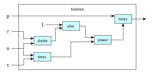
Given automata for different operations, we can combine them in various ways to make automata for more complex operations. Here’s a simple example:
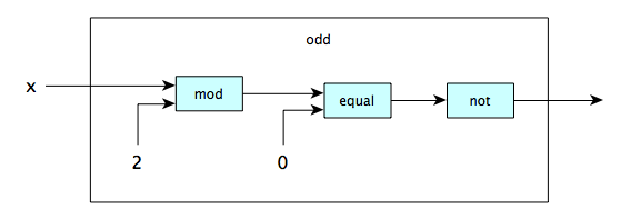
and a slightly larger one:
Where to Lean More
Check out the following sources for more information:
- Wikipedia article on Automata Theory
- A Short Introduction by some folks at Stanford in 2004
- The Sipser Theory of Computation Book
Recall Practice
Here are some questions useful for your spaced repetition learning. Many of the answers are not found on this page. Some will have popped up in lecture. Others will require you to do your own research.
- Automata Theory evolved form multiple fields of study. Name three. Mathematics, Engineering, and Psychology.
- What reasonable restrictions do we place on automata in Automata Theory? The machine must have a finite description, and the input must be a finite string of symbols from a fixed alphabet.
- What are two useful benefits from studying automata theory? It gives us (1) a framework to study the nature of computation and (2) insights into building real machines.
- What are the components of a Turing Machine? An infinite tape divided into cells, a tape head that can read and write symbols on the tape and move left or right, a finite set of states including a start state, an input alphabet, a tape alphabet (which includes at least the input alphabet plus a blank symbol), and a transition table that defines the machine's behavior.
- What does the transition table in a Turing Machine contain? It defines the machine's behavior by specifying, for each state and tape symbol, the next state, the symbol to write (if any), and the direction (if any) to move the tape head.
- What is an LBA? A Turing Machine with a tape of a fixed bounded length, and a transition table that can take into account what to do when at the tape boundaries.
- What is a PDA? A Turing Machine with a stack-based working memory separate from its read-only input tape, and in which the input is read from left-to-right with no way to go backwards.
- What is an FA? A Turing Machine with a finite tape consisting only of the input, and that reads the input from left to right without the ability to write or move backwards.
- What is a register machine? A machine with a finite number of registers, each holding a single unbounded natural number, and a program consisting of a list of instructions that operate on the registers.
- What are four dimensions on which we can vary the design of an abstract computing machine? Control, memory, output, and architecture.
- What are the two different behavioral variations of automata? Recognizers and transducers.
- What is the difference between a recognizer and a transducer? A recognizer outputs a YES or NO (or loops forever), while a transducer outputs a string (or loops forever).
- What do we call a recognizer that always stops, without looping forever? A decider.
- What are the three major control variations of automata? Instruction-set machines, rewrite machines, and state machines.
- What is a state machine? A machine that performs a computation by moving through states that indicate in which phase of the computation one is in.
- What is an instruction set machine? A machine that performs a computation by executing an (indexed) list of instructions. Jump instructions are allowed, so you can skip around the instruction list.
- What is a rewrite machine? A machine that performs a computation by applying a set of rewrite rules to a string.
- What are the two main ways to organize memory in automata theory? Tapes and registers.
- What are the two main architectural variations of automata, in terms of where control and data are located? Harvard Architecture and Von Neumann Architecture.
- What is the difference between the Harvard and von Neumann architectures? In the Harvard Architecture, instructions are stored separately from data, while in the von Neumann Architecture, instructions are stored together with data.
- What restrictions of Turing Machines correspond to RLGs, CFGs, and ENCGs? Finite Automata, Pushdown Automata, and Linear Bounded Automata, respectively.
- What kind of automaton accepts exactly the Regular Languages? Finite Automata (FA)
- What kind of automaton accepts exactly the Context Free Languages? Pushdown Automata (PDA)
- What kind of automaton accepts exactly the Type-1 Languages? Linear Bounded Automata (LBA)
- What kind of automaton accepts exactly the Recursively Enumerable Languages? Turing Machines (TMs)
- What is a finite language and what kinds of grammars generate them and what kinds of automata recognize them? A language with only a finite number of strings. They are generated by a grammar in which every rule maps the start symbol to a string in the language. They are recognized by a loop-free finite automaton.
- What is a regular language and what kinds of grammars generate them and what kinds of automata recognize them? A language in which strings can be recognized by processing them one symbol at a time, without backtracking, and without using additional memory. They are generated by a right-linear grammar. They are recognized by a finite automaton.
- What is a context-free language and what kinds of grammars generate them and what kinds of automata recognize them? A language in which strings can be recognized by processing them one symbol at a time, without backtracking, and by using only a simple stack for working memory. They are generated by a CFG. They are recognized by a PDA.
- What is a Type 1 language and what kinds of grammars generate them and what kinds of automata recognize them? A language in which strings can be recognized with fixed apriori bounds on working memory. They are generated by an ENCG. They are recognized by an LBA.
- What is the difference between a recursive and a recursively enumerable language? Recursive languages are exactly the decidable languages, that is, recognizable on a always-halting Turing Machine; recursively enumerable languages are partially decidable, meaning they can be recognized by a Turing Machine that always halts for YES answers but may loop forever on strings not in the language.
- Arrange R, CS, FINITE, RE, LR, CF, and REG in subset order. FINITE $\subset$ REG $\subset$ LR $\subset$ CFL $\subset$ CS $\subset$ R $\subset$ RE
- What is the difference between a deterministic and a nondeterministic automaton? Deterministic automata have only one possible transition to take when in a given configuration; nondeterministic automata have more than one.
- What is $RE \cap \textrm{co-}RE$? R
- Answering a YES-NO question on a Turing Machine is isomorphic to ________________ a language. Recognizing
- What is a “computable language”? A language that is recursively enumerable.
- What is the language class P? The set of languages that can be recognized by a deterministic TM in polynomial time.
- What is the language class NP? The set of languages that can be recognized by a TM in polynomial time.
- Why do we have language classes EXPTIME, EXPSPACE, and PSPACE, but no PTIME? Because PTIME is just another name for P.
- Who created the “Extended Chomsky Hierarchy” Diagram? Gabe Robins.
- According to Robins’s diagram, what is an example of a language that is decidable but cannot be decidable on an LBA? The language of all true propositions in Presburger Arithmetic.
- What is an example of a language that can be decided by a PDA but not by a deterministic PDA? Palindromes.
- Where do writers of compilers and interpreters most famously employ classic automata theory? In lexical analysis and parsing, where finite automata and pushdown automata are used, respectively.
- What are two programming languages that look like low-level automata? $\mathcal{P''}$ and Brainfuck.
- What are the eight instructions of Brainfuck and what do they do?
+: increment current cell-: decrement current cell,: read.: write<: move pointer left>: move pointer right[: jump past matching ] if current cell is 0]: jump back to matching [ if current cell is nonzero
Summary
We’ve covered:
- What automata theory is
- Some history of automata theory
- Various types of automata
- Relationship of automata theory with formal language theory
- Relationship of automata theory to computability theory