Recursion
What is Recursion?
Recursion is the process of repeating in a self-similar fashion. Objects that contain self-similar smaller copies (or near-copies) of themselves, or algorithms implemented with internal copies of themselves, are recursive.
Why is it Important?
Recursion is the way that the infinite can arise from a finite description. Or more usefully, it is the way that nature can use extremely compact representations for seemingly unbounded, complex phenomena.
Just look around. You see it everywhere:
- In nature
- In math
- In language
- In art
- In music
- In computer science
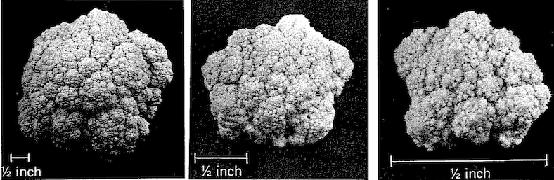
Recursion in Nature
Self-similarity occurs everywhere in nature. Zoom in on coastlines, clouds, broccoli, plants, or fire—at least for a few levels—and things look kind of the same.
Objects that are self-similar to many (even an infinite number of) levels are called Fractals and can be generated by repeated application of rather simple rules. See:
- Biomorphs
- Fractal Coastline Generator
- Fractal Terrain Generator
- Iterated Function Systems
- L-Systems
Recursion in Math
Math includes the study of patterns, so you don’t have to look too far to find recursion.
Recursive Definitions
Finite sets can be defined by enumerating their elements, but infinite sets cannot. We can build up infinite sets via rules. This is profound. Examples:
- Natural Number
- 0 is a natural number
- If $n$ is a natural number then so is $n+1$
- Nothing else is a natural number
- Odd integer
- 1 is an odd integer
- If $k$ is a an odd integer then so are $k+2$ and $k-2$
- Nothing else is an odd integer
- Palindrome
- A string of length 0 or 1 is a palindrome
- If $p$ is a palindrome and $c$ is a character then $cpc$ is a palindrome
- Nothing else is a palindrome
- Polynomial
- A real number is a polynomial
- The variable $x$ is a polynomial
- If $p$ and $q$ are polynomials then so are $p+q$, $p-q$, $pq$, $\frac{p}{q}$, and $(p)$.
- Nothing else is a polynomial
- Propositional Formula (PF)
- p, q, r, s, p', q', r', s', p'', ... are PFs
- If A and B are PFs then so are ~A, A ∧ B, A ∨ B, and (A).
- Nothing else is a PF
- Ancestors of x
- Mother(x) is in Ancestors(x)
- Father(x) is in Ancestors(x)
- if y is in Ancestors(x) then so are Mother(y) and Father(y)
- Nothing else is in Ancestors(x)
Note the importance of the "nothing else" clauses; without them your definitions are not unique.
Recursive Definitions vs. Circular Definitions
Proper recursive definitions must have a basis — a part of the definition that does not rely on the recursive step. Without a basis, you will likely get into serious trouble and end up with a useless circular definition.
- $x =_{\textrm{def}} \cos{x}$
- You got lucky here; this uniquely defines x 😅
- $x =_{\textrm{def}} x$
- ERROR: This is a circular definition, and therefore does not define anything! 👎🏽
- $x =_{\textrm{def}} x+1$
- ERROR: There's no such x, assuming we're taking about finite numbers here 🙅🏽
- $x =_{\textrm{def}} 6-x^2$
- DUBIOUS: x could be 2 or -3 🤔
Generating Sequences with Recursion
Infinite sequences are described finitely by giving a rule (or rules) for generating the next value in the sequence from previous ones. Examples:
- Fibonacci Numbers
- Definition: $F(0) = 0$, $F(1) = 1$, $F(n+2)$ = $F(n) + F(n+1)$
- Sequence: 0, 1, 1, 2, 3, 5, 8, 13, 21, 34, 55, 89, 144, 233, 377, ...
- Where seen: In nature
- Lucas Numbers
- Definition: $L(0) = 2$, $L(1) = 1$, $L(n+2) = L(n) + L(n+1)$
- Sequence: 2, 1, 3, 4, 7, 11, 18, 29, 47, 76, 123, 199, 322, 521, 843, ...
- Where seen: In nature
- Catalan Numbers
- Definition: $C(0) = 1$, $C(n+1) = \Sigma_{i=0}^n C(i)C(n-i)$
- Sequence: 1, 1, 2, 5, 14, 42, 132, 429, 1430, ...
- Where seen: In many counting scenarios
- Bell Numbers
- Definition: $B(0) = 1$, $B(n+1) = \Sigma_{i=0}^n {n \choose i} B(i)$
- Sequence: 1, 1, 2, 5, 15, 52, 203, 877, 4140, ...
- Where seen: The number of ways to partition a set
Nature and math often intersect. Take those Fibonacci Numbers: 0, 1, 1, 2, 3, 5, 8, 13, 21, 34, 55, 89, 144, 233, 377, .... These numbers are incredibly common in nature and worth knowing.
Now that you have memorized the beginning part of the sequence, treat yourself to Vi Hart’s amazing videos on these numbers in nature:
Inductive Proofs
Suppose you wanted to prove that every element in a recursively defined set had some property. You can't prove the property for each element because there are an infinite number of elements. But you can prove the property for the basis elements and then show that elements generated by the recursive rules maintain the property whenever the elements from which they were generated have the property.
Basis: The successor of 1 is 2 and 2 is divisible by 2. Step: Assume $k$ is odd and $k+1$ is divisible by 2. We have to show under these assumptions that (1) the successor of $k-2$ is divisible by 2 and (2) the successor of $k+2$ is divisible by 2. To prove (1) we note that the successor of $k-2$ is $k-1$ which is divisible by 2 because $k-1 = k+1-2$. To prove (2) note that the successor of $k+2$ is $k+3$ which is divisible by 2 because $k+3$ = $k+1+2$. This completes the proof.
Recursion in Language
Languages can exhibit recursion. For example, here is a grammar for a subset of English
(the | means “or,” the * means “zero-or-more,” and the ? means “zero-or-one.”):
S      ⟶  NP VP
NP     ⟶  (PN | DET ADJ* NOUN) (RP VP)?
VP     ⟶  IV | TV NP | DV NP PP | SV S
PP     ⟶  PREP NP
PN     ⟶  grace | tori | alan | she
DET    ⟶  a | the | his | her
NOUN   ⟶  doctor | dog | rat | girl | toy
RP     ⟶  who | that
ADJ    ⟶  blue | heavy | fast | new
PREP   ⟶  to | above | around | through
IV     ⟶  fell | jumped | swam
TV     ⟶  liked | knew | hit | missed
DV     ⟶  gave | threw | handed
SV     ⟶  dreamed | believed | thought | knew
Syntax diagrams, also known as recursive transition networks (RTNs) can be used too:
Where’s the recursion? Sentences contain verb phrases which contain sentences. Noun phrases contain verb phrases which contain verb phrases. Because of recursion we can make sentences of arbitrary length. Here's a simple example:
S
NP VP
DET NOUN RP VP VP
the NOUN RP VP VP
the dog RP VP VP
the dog that VP VP
the dog that SV S VP
the dog that thought S VP
the dog that thought NP VP VP
the dog that thought PN VP VP
the dog that thought grace VP VP
the dog that thought grace TV NP VP
the dog that thought grace hit NP VP
the dog that thought grace hit PN VP
the dog that thought grace hit alan VP
the dog that thought grace hit alan DV NP PP
the dog that thought grace hit alan threw NP PP
.
.
.
the dog that thought grace hit alan threw the new blue toy to the fast rat
Here's a construction that makes clear that you really can go on as long as you like:
S
NP VP
NP SV S
NP SV NP VP
NP SV NP SV S
NP SV NP SV NP VP
NP SV NP SV NP SV S
.
.
.
she dreamed she dreamed she dreamed she dreamed . . . she dreamed the dog swam
Further reading: A book chapter. A journal article.
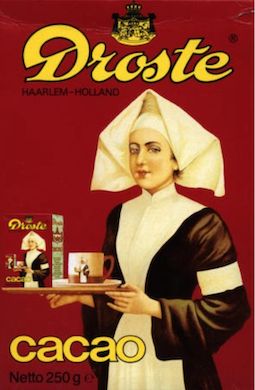
Recursion in Art
Sometimes you'll see a drawing contain a copy of itself. This is called the Droste Effect, named after the old Dutch cocoa brand that featured such an image on its packaging.
This effect is fun to animate:
There is an awesome play on this effect that is quite stunning—the picture inside the picture is the picture...itself! This appears in Escher's Print Gallery, though Escher did not draw the recursive effect himself. THis was done by de Smit and Lenstra in 2003.
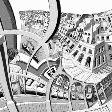
You’re encouraged to read the original paper, but if you want a beautiful analysis and “visual unpacking” on de Smit’s and Lenstra’s achievement, see this 3Blue1Brown video.
And there’s more in Section 4.2.3 in Chapter 4 of Maartje Schreuder’s Dissertation. (This excellent work covers a great deal about prosody in both music and art, with Chapter 4 focused specifically on recursion.)
Recursion in Music
Examples of recursive embeddings in music can be found in Section 4.2.4 in Chapter 4 of Maartje Schreuder’s Dissertation.
See also this short NPR story (which speaks more to fractals than to recursion directly).
Interested in the brain? Read this article from the journal Brain Structure and Function.
Now is a good opportunity to think about things that might be recursive or maybe just iterative. Watch the following video on Bach’s Endlessly Rising Canon. Do you think it is truly recursive or just iterative?
Recursion in Computer Science
We see recursion in both algorithms and in data.
“Recursion refers to a procedure that calls itself, or to a constituent that contains a constituent of the same kind.”
Recursive Algorithms
Here are three examples, out of the zillions known:
To walk n steps:
- If n <= 0, stop
- Take a single step
- Walk n-1 steps
To walk to the wall:
- If you are at the wall, stop
- Step
- Walk to the wall
To sort a list:
- If the list has zero or one elements, stop
- Sort the first half
- Sort the second half
- Merge the two sorted halves together, preserving the sort order
Recursive Functions
To write a recursive function, you must:
- have a base case
- ensure that each recursive call makes progress toward the base case
Here are some examples in Python:
# Here are a few examples of recursion.  The example functions were chosen
# because they are short and concise examples, not because they are good
# code.  In fact, nearly every method shown here is inferior to its
# iterative counterpart.

def factorial(n):
    return 1 if n == 0 else n * factorial(n - 1)

def sum_of_digits(n):
    if n < 0:
        return sum_of_digits(-n)
    elif n < 10:
        return n
    else:
        return sum_of_digits(n / 10) + (n % 10);

def is_palindrome(s):
    return len(s) <= 1 or (s[0] == s[-1] and is_palindrome(s[1:-1]))

def gcd(x, y):
    return x if y == 0 else gcd(y, x % y)
Understanding Recursive Functions
It is strongly suggested that you evaluate recursive functions by hand to get comfortable with them. For example:
factorial(4)
  = 4 * factorial(3)
  = 4 * (3 * factorial(2))
  = 4 * (3 * (2 * factorial(1)))
  = 4 * (3 * (2 * (1 * factorial(0))))
  = 4 * (3 * (2 * (1 * 1)))
  = 4 * (3 * (2 * 1))
  = 4 * (3 * 2)
  = 4 * 6
  = 24
sumOfDigits(-48729)
  = sumOfDigits(48279)
  = sumOfDigits(4827) + 9
  = (sumOfDigits(482) + 7) + 9
  = ((sumOfDigits(48) + 2) + 7) + 9
  = (((sumOfDigits(4) + 8) + 2) + 7) + 9
  = (((4 + 8) + 2) + 7) + 9
  = ((12 + 2) + 7) + 9
  = (14 + 7) + 9
  = 21 + 9
  = 30
gcd(444,93)
  = gcd(93,72)
  = gcd(72,21)
  = gcd(21,9)
  = gcd(9,3)
  = gcd(3,0)
  = 3
is_palindrome("racecar")
  = ('r' == 'r') and is_palindrome("aceca")
  = true and is_palindrome("aceca")
  = is_palindrome("aceca")
  = ('a' == 'a') and is_palindrome("cec")
  = true and is_palindrome("cec")
  = is_palindrome("cec")
  = ('c' == 'c') and is_palindrome("a")
  = true and is_palindrome("a")
  = is_palindrome("a")
  = true
Efficiency
Note that just because some functions are described recursively doesn't mean programmers should write them as such. They might be slow! Look at the factorial and sum-of-digits examples above. As we make recursive calls, the runtime system is stacking up partial results, requiring lots of memory to remember the partial results, so they can be combined only after the last recursive call. These partial results are stored in the system stack, and if the recursion goes to deep, the program crashes with a stack overflow error.
One way to fix problematic issues like factorial and sum-of-digits recursion is to just use a loop, which do not require tons of partial results to be stacked up! Instead, the results are combined as we compute. Using loops gives us what we call iterative solutions:
def factorial(n):
    product = 1
    for i in range(n):
        product *= i
    return product

def sum_of_digits(n):
    sum = 0
    remaining = abs(n)
    while remaining > 0:
        sum += remaining % 10
        remaining //= 10
    return sum if n > 0 else -sum
Now note the gcd example is okay: no partial results are stacked up. The function returns a recursive call itself. This is called tail recursion and it is good.
Now what about the palindrome example. It is tail recursive, and that part is okay, but unless we know that the underlying implementation of our programming language is not manufacturing new string objects during each recursive call, we could be in danger.
Think about whether the recursive formulations are easier or harder to come up with that the iterative versions.
Efficiency Horrors
Often needless recursion turns linear into exponential complexity! Remember the Fibonacci sequence?
$F(0) = 0 \\ F(1) = 1 \\ F(n+2) = F(n) + F(n+1)$What if we programmed this directly into a function? IT WOULD BE A DISASTER! 😱
# HORRIFIC CODE for computing the nth Fibonacci Number. NEVER write code like this.
def fib(n):
    return n if n <= 1 else fib(n-2) + fib(n-1)
You can see why this inefficient:
fib(5) = fib(4) + fib(3)
  = (fib(3) + fib(2)) + fib(3)
  = ((fib(2) + fib(1)) + fib(2)) + fib(3)
  = (((fib(1) + fib(0)) + fib(1)) + fib(2)) + fib(3)
  = (((1 + fib(0)) + fib(1)) + fib(2)) + fib(3)
  = (((1 + 0) + fib(1)) + fib(2)) + fib(3)
  = ((1 + fib(1)) + fib(2)) + fib(3)
  = ((1 + 1) + fib(2)) + fib(3)
  = (2 + fib(2)) + fib(3)
  = (2 + (fib(1) + fib(0))) + fib(3)
  = (2 + (1 + fib(0))) + fib(3)
  = (2 + (1 + 0)) + fib(3)
  = (2 + 1) + fib(3)
  = 3 + fib(3)
  = 3 + (fib(2) + fib(1))
  = 3 + ((fib(1) + fib(0)) + fib(1))
  = 3 + ((1 + fib(0)) + fib(1))
  = 3 + ((1 + 0) + fib(1))
  = 3 + (1 + fib(1))
  = 3 + (1 + 1)
  = 3 + 2
  = 5
BTW it wil make 25 calls to fib just to determine that the value of fib(6) is 13, 41 calls to get the value of fib(7), and 535,821,591 calls to get fib(40). The problem is that we are doing many of the sub-calls multiple times!
Here is another disastrous example. The binomial coefficients also show up a lot. You might have seen them in Pascal’s Triangle:
                1
              1   1
            1   2   1
          1   3   3   1
        1   4   6   4   1
      1   5  10  10   5   1
    1   6  15  20  15   6   1
  1   7  21  35  35  21   7   1
1   8  28  56  70  56  28   8   1
Here’s the rule:
$ C(n, k) = \begin{cases} 1 & \mathrm{if}\;k = 0 \\ 1 & \mathrm{if}\;k = n \\ C(n-1,k)+C(n-1,k-1) & \mathrm{if}\;1 \leq k \leq n-1 \end{cases} $Unfortunately, as before, turning this into code directly will generate a lot of duplicated work in the multi-way recursion. But it is not super clear how to solve this iteratively. Wouldn’t it be cool if we could write the recursive algorithm, but each time we’ve need to do a calculation we’ve seen before, we can re-use the value we computed before?
Memoization
Whenever multi-way recursion has repetition, we should re-use computations we’ve seen before. This is called memoization.
Here’s the idea. When calling a multi-way recursive function, first check to see if you’ve seen those arguments before and already computed a result. If so, returned the cached result. If not, execute the function, and just before returning, save your result in the cache.
So the horrific version of the C function we saw above is:
def c(n,k):
    return 1 if k <= 0 or k >= n else c(n-1,k-1) + c(n-1,k)
When I tried this on my MacBook Air, it took 33.4 seconds to compute c(30,15) and it took 161 sec to compute C(32,16). Run times roughly double every time we increase $n$ by 1. So we will need several hours to compute C(40,20) and many, many years to compute C(50,25).
A hand-memoized version is:
def c(n, k):
    cache = {}
    def cm(n, k):
        if (n, k) not in cache:
            cache[(n,k)] = 1 if k <= 0 or k >= n else cm(n-1,k-1) + cm(n-1,k)
        return cache[(n,k)]
    return cm(n, k)
On my laptop, it took 0.000549907 sec to do C(50,25). Also C(200,100), which never would have finished without memoization in the lifetime of our universe, computed the result in 0.00693 seconds.
ARE YOU IMPRESSED?
In practice, you would employ a decorator for memoization, then blissfully write elegant multi-way recursion and be at peace knowing memoization is happening behind the scenes. This approach sure beats that “bottom-up” table-based dynamic programming mechanism you might have run across in your studies. IMHO anyway.
def memoized(f):
    cache = {}
    def wrapper(*args):
        if args not in cache:
            cache[args] = f(*args)
        return cache[args]
    return wrapper
Here’s our function with its decorator:
@memoized
def c(n,k):
    return 1 if k <= 0 or k >= n else c(n-1,k-1) + c(n-1,k)
The real benefit of the decorator is that it can be applied to any multi-way recursive function (assuming the arguments can be used as dictionary keys). Some examples:
@memoized
def fib(n):
    """Return the nth Fibonacci Number"""
    return n if n <= 1 else fib(n-2) + fib(n-1)
@memoized
def minimum_coins(amount, denominations):
    """Return the minimum number of coins needed to make an amount where
    the denominations are stored in a list which must contain a 1, or the
    result of this function is undefined."""
    min_so_far = amount
    for denomination in denominations:
        if denomination == amount:
            return 1
        elif denomination < amount:
            min_so_far = min(min_so_far, 1+minimum_coins(amount-denomination, denominations))
    return min_so_far
minimum_coins would be made when calling the method with the arguments 97 and [4, 1, 6, 23, 11]?
When is memoization needed?Take care to use it only for multi-way recursion when you are likely to see subproblems reappear. It the subproblems never overlap, you will not get any benefit from the technique.
Useful Examples of Recursion
Recursion is most useful when:
- You can't easily replace it with a simple loop because the structure is being processed "backwards"
- You need to do a multi-way recursion but you are careful to avoid duplicating work
- You are implementing and algorithm using a known paradigm like backtracking or dynamic programming
- The recursion is a tail recursion which you know your compiler will optimize away
Multi-way recursion without duplication shows up naturally in backtracking algorithms (like maze solving) or divide-and-conquer algorithms (like merge sort and quick sort). It’s generally fine to just write these recursively.
For examples, see the notes on Backtracking.
For something really cool, checkout this list of a number of “sophisticated” algorithms that employ recursion.
Recursive Datatypes
Often you'll have a datatype whose components are (references to) objects of the datatype itself. For example, a person might have a name and an (optional) mother and an (optional) father. The mother and father are people! Recursion!

Most of the methods operating on such an object would naturally be recursive:
def length_of_known_maternal_line(p) {
    return 0 if p is None else 1 + length_of_known_maternal_line(p.mom);
}
When defining recursive datatypes, you use a form similar to those we saw above with mathematical recursive definitions. Here are two examples:
A list is either empty or an element attached to the front of a list.
A tree is either empty or an element attached to zero or more trees (called its subtrees).
When a data type is defined recursively, the methods that operate on them will naturally be recursive. They often just write themselves!
Recursive Computers
What better way to close a discussion of recursion in computer science than with this important insight from Alan Kay:
Bob Barton, the main designer of the B5000 and a professor at Utah had said in one of his talks a few days earlier: "The basic principle of recursive design is to make the parts have the same power as the whole." For the first time I thought of the whole as the entire computer and wondered why anyone would want to divide it up into weaker things called data structures and procedures. Why not divide it up into little computers, as time sharing was starting to? But not in dozens. Why not thousands of them, each simulating a useful structure?
— Alan Kay, The Early History of Smalltalk
Fascinating, right?
Summary
We’ve covered:
- What is Recursion?
- Why is it Important?
- Recursion in Nature
- Recursion in Math
- Recursion in Language
- Syntax Diagrams
- Recursion in Art
- Recursion in Music
- Recursion in Computer Science
- Recursive algorithms and functions
- Efficiency concerns with recursion
- Tips for when using recursion is okay
- The usefulness of recursive datatypes